

100
M. Lucas et al.
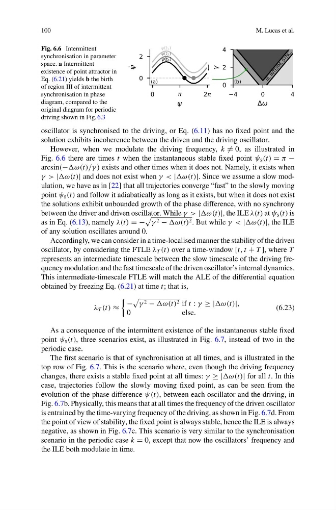
Fig. 6.6 Intermittent
synchronisation in parameter
space. a Intermittent
existence of point attractor in
Eq. (6.21) yields b the birth
of region III of intermittent
synchronisation in phase
diagram, compared to the
original diagram for periodic
driving shown in Fig. 6.3
oscillator is synchronised to the driving, or Eq. (6.11) has no fixed point and the
solution exhibits incoherence between the driven and the driving oscillator.
However, when we modulate the driving frequency, k = 0, as illustrated in
Fig. 6.6 there are times t when the instantaneous stable fixed point ψ s (t) = π −
arcsin(− ) exists and other times when it does not. Namely, it exists when
γ > | and does not exist when γ < | Since we assume a slow modulation, we have as in [22] that all trajectories converge “fast” to the slowly moving
point ψ s (t) and follow it adiabatically as long as it exists, but when it does not exist
the solutions exhibit unbounded growth of the phase difference, with no synchrony
between the driver and driven oscillator. While γ > | the ILE λ(t) at ψ s (t) is
as in Eq. (6.13), namely λ(t) = −
γ 2 − ω(t) 2 . But while γ < | the ILE
of any solution oscillates around 0.
Accordingly, we can consider in a time-localised manner the stability of the driven
oscillator, by considering the FTLE λ T (t) over a time-window [t, t + T ], where T
represents an intermediate timescale between the slow timescale of the driving frequency modulation and the fast timescale of the driven oscillator’s internal dynamics.
This intermediate-timescale FTLE will match the ALE of the differential equation
obtained by freezing Eq. (6.21) at time t; that is,
λ T (t) ≈
−
γ 2 − 2 if t : γ ≥ |ω(t)|,
0
e l s e .
(6.23)
As a consequence of the intermittent existence of the instantaneous stable fixed
point ψ s (t), three scenarios exist, as illustrated in Fig. 6.7, instead of two in the
periodic case.
The first scenario is that of synchronisation at all times, and is illustrated in the
top row of Fig. 6.7. This is the scenario where, even though the driving frequency
changes, there exists a stable fixed point at all times: γ ≥ |ω(t)| for all t. In this
case, trajectories follow the slowly moving fixed point, as can be seen from the
evolution of the phase difference ψ(t), between each oscillator and the driving, in
Fig. 6.7b. Physically, this means that at all times the frequency of the driven oscillator
is entrained by the time-varying frequency of the driving, as shown in Fig. 6.7d. From
the point of view of stability, the fixed point is always stable, hence the ILE is always
negative, as shown in Fig. 6.7c. This scenario is very similar to the synchronisation
scenario in the periodic case k = 0, except that now the oscillators’ frequency and
the ILE both modulate in time.
M. Lucas et al.
Fig. 6.6 Intermittent
synchronisation in parameter
space. a Intermittent
existence of point attractor in
Eq. (6.21) yields b the birth
of region III of intermittent
synchronisation in phase
diagram, compared to the
original diagram for periodic
driving shown in Fig. 6.3
oscillator is synchronised to the driving, or Eq. (6.11) has no fixed point and the
solution exhibits incoherence between the driven and the driving oscillator.
However, when we modulate the driving frequency, k = 0, as illustrated in
Fig. 6.6 there are times t when the instantaneous stable fixed point ψ s (t) = π −
arcsin(− ) exists and other times when it does not. Namely, it exists when
γ > | and does not exist when γ < | Since we assume a slow modulation, we have as in [22] that all trajectories converge “fast” to the slowly moving
point ψ s (t) and follow it adiabatically as long as it exists, but when it does not exist
the solutions exhibit unbounded growth of the phase difference, with no synchrony
between the driver and driven oscillator. While γ > | the ILE λ(t) at ψ s (t) is
as in Eq. (6.13), namely λ(t) = −
γ 2 − ω(t) 2 . But while γ < | the ILE
of any solution oscillates around 0.
Accordingly, we can consider in a time-localised manner the stability of the driven
oscillator, by considering the FTLE λ T (t) over a time-window [t, t + T ], where T
represents an intermediate timescale between the slow timescale of the driving frequency modulation and the fast timescale of the driven oscillator’s internal dynamics.
This intermediate-timescale FTLE will match the ALE of the differential equation
obtained by freezing Eq. (6.21) at time t; that is,
λ T (t) ≈
−
γ 2 − 2 if t : γ ≥ |ω(t)|,
0
e l s e .
(6.23)
As a consequence of the intermittent existence of the instantaneous stable fixed
point ψ s (t), three scenarios exist, as illustrated in Fig. 6.7, instead of two in the
periodic case.
The first scenario is that of synchronisation at all times, and is illustrated in the
top row of Fig. 6.7. This is the scenario where, even though the driving frequency
changes, there exists a stable fixed point at all times: γ ≥ |ω(t)| for all t. In this
case, trajectories follow the slowly moving fixed point, as can be seen from the
evolution of the phase difference ψ(t), between each oscillator and the driving, in
Fig. 6.7b. Physically, this means that at all times the frequency of the driven oscillator
is entrained by the time-varying frequency of the driving, as shown in Fig. 6.7d. From
the point of view of stability, the fixed point is always stable, hence the ILE is always
negative, as shown in Fig. 6.7c. This scenario is very similar to the synchronisation
scenario in the periodic case k = 0, except that now the oscillators’ frequency and
the ILE both modulate in time.