

6 Synchronisation and Non-autonomicity
99
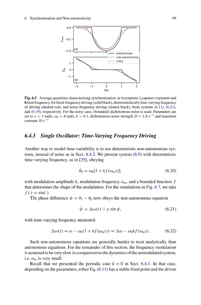
Fig. 6.5 Average quantities characterising synchronisation. a Asymptotic Lyapunov exponent and
b beat frequency, for fixed-frequency driving (solid black), deterministically time-varying frequency
of driving (dashed red), and noisy-frequency driving (dotted black), from systems (6.11), (6.21),
and (6.19), respectively. For the noisy case, (bounded) dichotomous noise is used. Parameters are
set to γ = 1 rad/s, ω 0 = 4 rad/s, k = 0.1, dichotomous noise strength D = 1.6 s −1 and transition
constant 10 s −1
6.4.3 Single Oscillator: Time-Varying Frequency Driving
Another way to model time-variability is to use deterministic non-autonomous systems, instead of noise as in Sect. 6.4.2. We present system (6.9) with deterministic
time-varying frequency, as in [35], obeying
˙
θ 0 = ω 0 [1 + k f (ω m t)],
(6.20)
with modulation amplitude k, modulation frequency ω m , and a bounded function f
that determines the shape of the modulation. For the simulations in Fig. 6.7, we take
f (·) = sin(·).
The phase difference ψ = θ 1 − θ 0 now obeys the non-autonomous equation
˙
ψ = + γ sin ψ,
(6.21)
with time-varying frequency mismatch
ω(t) = ω − ω 0 (1 + k f (ω m t)) = − ω 0 k f (ω m t).
(6.22)
Such non-autonomous equations are generally harder to treat analytically than
autonomous equations. For the remainder of this section, the frequency modulation
is assumed to be very slow in comparison to the dynamics of the unmodulated system,
i.e. ω m is very small.
Recall that we presented the periodic case k = 0 in Sect. 6.4.1. In that case,
depending on the parameters, either Eq. (6.11) has a stable fixed point and the driven
99
Fig. 6.5 Average quantities characterising synchronisation. a Asymptotic Lyapunov exponent and
b beat frequency, for fixed-frequency driving (solid black), deterministically time-varying frequency
of driving (dashed red), and noisy-frequency driving (dotted black), from systems (6.11), (6.21),
and (6.19), respectively. For the noisy case, (bounded) dichotomous noise is used. Parameters are
set to γ = 1 rad/s, ω 0 = 4 rad/s, k = 0.1, dichotomous noise strength D = 1.6 s −1 and transition
constant 10 s −1
6.4.3 Single Oscillator: Time-Varying Frequency Driving
Another way to model time-variability is to use deterministic non-autonomous systems, instead of noise as in Sect. 6.4.2. We present system (6.9) with deterministic
time-varying frequency, as in [35], obeying
˙
θ 0 = ω 0 [1 + k f (ω m t)],
(6.20)
with modulation amplitude k, modulation frequency ω m , and a bounded function f
that determines the shape of the modulation. For the simulations in Fig. 6.7, we take
f (·) = sin(·).
The phase difference ψ = θ 1 − θ 0 now obeys the non-autonomous equation
˙
ψ = + γ sin ψ,
(6.21)
with time-varying frequency mismatch
ω(t) = ω − ω 0 (1 + k f (ω m t)) = − ω 0 k f (ω m t).
(6.22)
Such non-autonomous equations are generally harder to treat analytically than
autonomous equations. For the remainder of this section, the frequency modulation
is assumed to be very slow in comparison to the dynamics of the unmodulated system,
i.e. ω m is very small.
Recall that we presented the periodic case k = 0 in Sect. 6.4.1. In that case,
depending on the parameters, either Eq. (6.11) has a stable fixed point and the driven