

6 p-Wave Superconductivity and d-Vector Representation
169
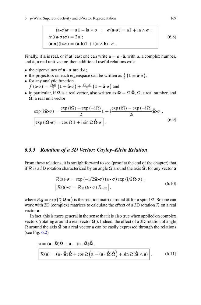
(a·σ )σ = a1 − ia ∧ σ ; σ (a·σ ) = a1 + ia ∧ σ ;
tr((a·σ )σ ) = 2 a ;
(a·σ )(b·σ ) = (a·b)1 + i(a ∧ b) · σ .
(6.8)
Finally, if a is real, or if at least one can write a = a · ˆ
a, with a, a complex number,
and ˆ
a, a real unit vector, then additional useful relations exist
• the eigenvalues of a · σ are ±a;
• the projectors on each eigenspace can be written as
1
2
1 ± ˆ
a·σ
;
• for any analytic function
f (a·σ ) =
f (a)
2
1 + ˆ
a·σ
+
f (−a)
2
1 − ˆ
a·σ
and
• in particular, if is a real vector, also written as = ˆ
, , a real number, and
ˆ
, a real unit vector
exp (i·σ ) =
exp (i) + exp (−i)
2
1 + i
exp (i) − exp (−i)
2i
ˆ
·σ ,
exp (i·σ ) = cos 1 + i sin ˆ
·σ .
(6.9)
6.3.3 Rotation of a 3D Vector: Cayley–Klein Relation
From these relations, it is straightforward to see (proof at the end of the chapter) that
if R is a 3D rotation characterized by an angle around the axis ˆ
, for any vector a
R(a)·σ = exp (−i/2·σ ) (a · σ ) exp (i/2·σ ) ,
R(a)·σ = R (a · σ ) R − ,
(6.10)
where R = exp
−i
2
·σ
is the rotation matrix around for a spin 1/2. So one can
work with 2D (complex) matrices to calculate the effect of a 3D rotation R on a real
vector a.
In fact, this is more general in the sense that it is also true when applied on complex
vectors (rotating around a real vector ). Indeed, the effect of a 3D rotation of angle
around the axis ˆ
on a real vector a can be easily expressed through the relations
(see Fig. 6.2)
a = (a · ˆ
) ˆ
+ a − (a · ˆ
) ˆ
,
R(a) = (a · ˆ
) ˆ
+ cos
a − (a · ˆ
) ˆ
+ sin ( ˆ
∧ a) .
(6.11)
169
(a·σ )σ = a1 − ia ∧ σ ; σ (a·σ ) = a1 + ia ∧ σ ;
tr((a·σ )σ ) = 2 a ;
(a·σ )(b·σ ) = (a·b)1 + i(a ∧ b) · σ .
(6.8)
Finally, if a is real, or if at least one can write a = a · ˆ
a, with a, a complex number,
and ˆ
a, a real unit vector, then additional useful relations exist
• the eigenvalues of a · σ are ±a;
• the projectors on each eigenspace can be written as
1
2
1 ± ˆ
a·σ
;
• for any analytic function
f (a·σ ) =
f (a)
2
1 + ˆ
a·σ
+
f (−a)
2
1 − ˆ
a·σ
and
• in particular, if is a real vector, also written as = ˆ
, , a real number, and
ˆ
, a real unit vector
exp (i·σ ) =
exp (i) + exp (−i)
2
1 + i
exp (i) − exp (−i)
2i
ˆ
·σ ,
exp (i·σ ) = cos 1 + i sin ˆ
·σ .
(6.9)
6.3.3 Rotation of a 3D Vector: Cayley–Klein Relation
From these relations, it is straightforward to see (proof at the end of the chapter) that
if R is a 3D rotation characterized by an angle around the axis ˆ
, for any vector a
R(a)·σ = exp (−i/2·σ ) (a · σ ) exp (i/2·σ ) ,
R(a)·σ = R (a · σ ) R − ,
(6.10)
where R = exp
−i
2
·σ
is the rotation matrix around for a spin 1/2. So one can
work with 2D (complex) matrices to calculate the effect of a 3D rotation R on a real
vector a.
In fact, this is more general in the sense that it is also true when applied on complex
vectors (rotating around a real vector ). Indeed, the effect of a 3D rotation of angle
around the axis ˆ
on a real vector a can be easily expressed through the relations
(see Fig. 6.2)
a = (a · ˆ
) ˆ
+ a − (a · ˆ
) ˆ
,
R(a) = (a · ˆ
) ˆ
+ cos
a − (a · ˆ
) ˆ
+ sin ( ˆ
∧ a) .
(6.11)