

168
J.-P. Brison
But it would not do the job: the module would be fine, but the direction of V and so
its transformation under rotations of the axis would be meaningless, for example, for
the same quantization axis a pure | ↑↑↑ or | ↓↓↓ state would lead to perpendicular
vectors. Or equivalently, taking an opposite direction of the quantization axis would
yield perpendicular vector representations. This is clearly not what is expected from
a vector behaviour. The problem stems from the fact that one needs to make a link
between the spin state [SU(2)] and three-dimensional vectors. The good news is
that this problem has been solved long ago in classical mechanics, with the Cayley–
Klein representation, which aimed at simplifying the calculation of rotation effects;
in real space, a matrix rotation is a 3 × 3 matrix; however, it is fully characterized
by only three angles (the Euler angles for example); so, in principle, a 2 × 2 matrix,
with four parameters, should be more than enough. The Cayley–Klein representation
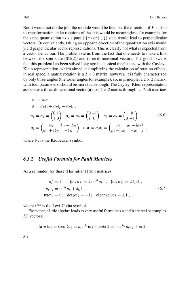
associates a three-dimensional vector (a) to a 2 × 2 matrix through … Pauli matrices
a → a·σ ,
σ = σ 1 e x + σ 2 e y + σ 3 e z ,
σ 1 = σ x =
0 1
1 0
σ 2 = σ y =
0 −i
i 0
σ 3 = σ z =
1 0
0 −1
,
σ i =
δ 3i
δ 1i − iδ 2i
δ 1i + iδ 2i −δ 3i
a·σ = a i σ i =
a 3
a 1 − ia 2
a 1 + ia 2 −a 3
,
(6.6)
where δ i j is the Kronecker symbol.
6.3.2 Useful Formula for Pauli Matrices
As a reminder, for these (Hermitian) Pauli matrices
σ
2
i = 1 ; [σ i , σ j ] = 2i
i jk
σ k ; {σ i , σ j } = 2 δ i j 1 ,
σ i σ j = i
i jk
σ k + δ i j 1 ,
tr(σ i ) = 0; det(σ i ) = −1; eigenvalues = ±1 ,
(6.7)
where
i jk is the Levi-Civita symbol.
From that, a little algebra leads to very useful formulae (a and b are real or complex
3D vectors)
(a·σ )σ k = (a i σ i )σ k = a i
ik j iσ j + a i δ ik 1 = −i
ki j a i σ j + a k 1 .
So
J.-P. Brison
But it would not do the job: the module would be fine, but the direction of V and so
its transformation under rotations of the axis would be meaningless, for example, for
the same quantization axis a pure | ↑↑↑ or | ↓↓↓ state would lead to perpendicular
vectors. Or equivalently, taking an opposite direction of the quantization axis would
yield perpendicular vector representations. This is clearly not what is expected from
a vector behaviour. The problem stems from the fact that one needs to make a link
between the spin state [SU(2)] and three-dimensional vectors. The good news is
that this problem has been solved long ago in classical mechanics, with the Cayley–
Klein representation, which aimed at simplifying the calculation of rotation effects;
in real space, a matrix rotation is a 3 × 3 matrix; however, it is fully characterized
by only three angles (the Euler angles for example); so, in principle, a 2 × 2 matrix,
with four parameters, should be more than enough. The Cayley–Klein representation
associates a three-dimensional vector (a) to a 2 × 2 matrix through … Pauli matrices
a → a·σ ,
σ = σ 1 e x + σ 2 e y + σ 3 e z ,
σ 1 = σ x =
0 1
1 0
σ 2 = σ y =
0 −i
i 0
σ 3 = σ z =
1 0
0 −1
,
σ i =
δ 3i
δ 1i − iδ 2i
δ 1i + iδ 2i −δ 3i
a·σ = a i σ i =
a 3
a 1 − ia 2
a 1 + ia 2 −a 3
,
(6.6)
where δ i j is the Kronecker symbol.
6.3.2 Useful Formula for Pauli Matrices
As a reminder, for these (Hermitian) Pauli matrices
σ
2
i = 1 ; [σ i , σ j ] = 2i
i jk
σ k ; {σ i , σ j } = 2 δ i j 1 ,
σ i σ j = i
i jk
σ k + δ i j 1 ,
tr(σ i ) = 0; det(σ i ) = −1; eigenvalues = ±1 ,
(6.7)
where
i jk is the Levi-Civita symbol.
From that, a little algebra leads to very useful formulae (a and b are real or complex
3D vectors)
(a·σ )σ k = (a i σ i )σ k = a i
ik j iσ j + a i δ ik 1 = −i
ki j a i σ j + a k 1 .
So