

110
H. Elnaggar et al.
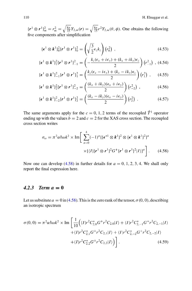
{r
1
⊗ r
1
}
2
m = r
2
m =
8π
15
Y 2,m (r) =
8π
15
r
2 Y 2,m (θ, φ). One obtains the following
five components after simplification
{
1
⊗ k
1
}
2
0 {r
1
⊗ r
1
}
2
0 =
3
2
z k z
r
2
0
,
(4.53)
{
1
⊗ k
1
}
2
1 {r
1
⊗ r
1
}
2
−1 =
−
k z (( x + i y ) + (k x + ik y )) z
2
r
2
−1
, (4.54)
{
1
⊗ k
1
}
2
−1 {r
1
⊗ r
1
}
2
1 =
k z (( x − i y ) + (k x − ik y )) z
2
r
2
1
,
(4.55)
{
1
⊗ k
1
}
2
2 {r
1
⊗ r
1
}
2
−2 =
(k x + ik y )(( x + i y )
2
r
2
−2
,
(4.56)
{
1
⊗ k
1
}
2
−2 {r
1
⊗ r
1
}
2
2 =
(k x − ik y )(( x − i y )
2
r
2
2
.
(4.57)
The same arguments apply for the c = 0, 1, 2 terms of the recoupled ˆ
T
† operator
ending up with the values b = 2 and c = 2 for the XAS cross section. The recoupled
cross section writes
σ ω = π
2
αωk
2
× Im
4
a=0
(−1)
a
{{
∗1
⊗ k
1
}
2
⊗ {
1
⊗ k
1
}
2
}
a
×{{I |{r
1
⊗ r
1
}
2 G
+
{r
1
⊗ r
1
}
2
|I }
a
.
(4.58)
Now one can develop (4.58) in further details for a = 0, 1, 2, 3, 4. We shall only
report the final expression here.
4.2.3 Term a = 0
Let us substitute a = 0 in (4.58). This is the zero rank of the tensor, σ (0, 0), describing
an isotropic spectrum
σ (0, 0) = π
2
αωk
2
× Im
1
10
I |r
2 C
∗
2,0 G
+ r
2 C 2,0 |I + +I |r
2 C
∗
2,−1 G
+ r
2 C 2,−1 |I
++I |r
2 C
∗
2,1 G
+ r
2 C 2,1 |I + +I |r
2 C
∗
2,−2 G
+ r
2 C 2,−2 |I
++I |r
2 C
∗
2,2 G
+ r
2 C 2,2 |I
.
(4.59)
H. Elnaggar et al.
{r
1
⊗ r
1
}
2
m = r
2
m =
8π
15
Y 2,m (r) =
8π
15
r
2 Y 2,m (θ, φ). One obtains the following
five components after simplification
{
1
⊗ k
1
}
2
0 {r
1
⊗ r
1
}
2
0 =
3
2
z k z
r
2
0
,
(4.53)
{
1
⊗ k
1
}
2
1 {r
1
⊗ r
1
}
2
−1 =
−
k z (( x + i y ) + (k x + ik y )) z
2
r
2
−1
, (4.54)
{
1
⊗ k
1
}
2
−1 {r
1
⊗ r
1
}
2
1 =
k z (( x − i y ) + (k x − ik y )) z
2
r
2
1
,
(4.55)
{
1
⊗ k
1
}
2
2 {r
1
⊗ r
1
}
2
−2 =
(k x + ik y )(( x + i y )
2
r
2
−2
,
(4.56)
{
1
⊗ k
1
}
2
−2 {r
1
⊗ r
1
}
2
2 =
(k x − ik y )(( x − i y )
2
r
2
2
.
(4.57)
The same arguments apply for the c = 0, 1, 2 terms of the recoupled ˆ
T
† operator
ending up with the values b = 2 and c = 2 for the XAS cross section. The recoupled
cross section writes
σ ω = π
2
αωk
2
× Im
4
a=0
(−1)
a
{{
∗1
⊗ k
1
}
2
⊗ {
1
⊗ k
1
}
2
}
a
×{{I |{r
1
⊗ r
1
}
2 G
+
{r
1
⊗ r
1
}
2
|I }
a
.
(4.58)
Now one can develop (4.58) in further details for a = 0, 1, 2, 3, 4. We shall only
report the final expression here.
4.2.3 Term a = 0
Let us substitute a = 0 in (4.58). This is the zero rank of the tensor, σ (0, 0), describing
an isotropic spectrum
σ (0, 0) = π
2
αωk
2
× Im
1
10
I |r
2 C
∗
2,0 G
+ r
2 C 2,0 |I + +I |r
2 C
∗
2,−1 G
+ r
2 C 2,−1 |I
++I |r
2 C
∗
2,1 G
+ r
2 C 2,1 |I + +I |r
2 C
∗
2,−2 G
+ r
2 C 2,−2 |I
++I |r
2 C
∗
2,2 G
+ r
2 C 2,2 |I
.
(4.59)