

98
H. Elnaggar et al.
depending only on the experimental conditions (k, ). Such a geometric and fully
decoupled expression is useful: (i) to disentangle the properties of the sample from
those of the measurement; (ii) to determine specific experimental arrangements aiming at the observation of specific sample properties; (iii) to provide the most convenient starting point to investigate the reduction of the number of fundamental spectra
due to crystal symmetries.
4.2.1 The Case of Electric Dipole Transitions
The first step is to build rank one spherical tensors from the vectors appearing in the
transition operator. The polarization vector = [ x , , y , , z ] can be written as a spherical tensor
1 with components
1
−1 =
x −i y
√
2
,
1
1 = −
x +i y
√
2
, and
1
0 = z . Similarly,
the position spherical tensor, r
1 , can be constructed. In the following we shall use
the following notation for the coupling of spherical tensors P
a and Q
b of ranks a
and b into a spherical tensor of rank c
{ P
a
⊗ Q
b
}
c
γ =
a
α=−a
b
α=−b
(aαbβ|cγ )P
a
α Q
b
β ,
(4.24)
with (aαbβ|cγ ) being the Clebsch–Gordan coefficients. Therefore,
P
a
· Q
a
=
a
α=−a
(−1)
α P
a
−α Q
a
α = (−1)
a
√
2a + 1{ P
a
⊗ Q
a
}
0
.
(4.25)
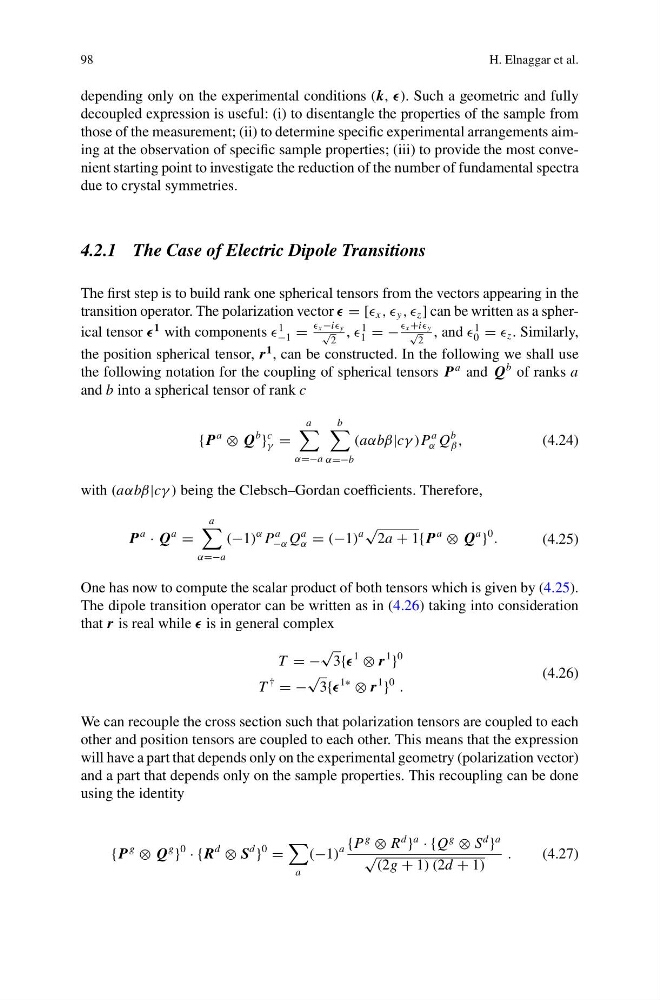
One has now to compute the scalar product of both tensors which is given by (4.25).
The dipole transition operator can be written as in (4.26) taking into consideration
that r is real while is in general complex
T = −
√
3{
1
⊗ r
1
}
0
T
†
= −
√
3{
1∗
⊗ r
1
}
0
.
(4.26)
We can recouple the cross section such that polarization tensors are coupled to each
other and position tensors are coupled to each other. This means that the expression
will have a part that depends only on the experimental geometry (polarization vector)
and a part that depends only on the sample properties. This recoupling can be done
using the identity
{ P
g
⊗ Q
g
}
0
· {R
d
⊗ S
d
}
0
=
a
(−1)
a {P
g
⊗ R
d
}
a
· {Q
g
⊗ S
d
}
a
√ (2g + 1) (2d + 1)
.
(4.27)
H. Elnaggar et al.
depending only on the experimental conditions (k, ). Such a geometric and fully
decoupled expression is useful: (i) to disentangle the properties of the sample from
those of the measurement; (ii) to determine specific experimental arrangements aiming at the observation of specific sample properties; (iii) to provide the most convenient starting point to investigate the reduction of the number of fundamental spectra
due to crystal symmetries.
4.2.1 The Case of Electric Dipole Transitions
The first step is to build rank one spherical tensors from the vectors appearing in the
transition operator. The polarization vector = [ x , , y , , z ] can be written as a spherical tensor
1 with components
1
−1 =
x −i y
√
2
,
1
1 = −
x +i y
√
2
, and
1
0 = z . Similarly,
the position spherical tensor, r
1 , can be constructed. In the following we shall use
the following notation for the coupling of spherical tensors P
a and Q
b of ranks a
and b into a spherical tensor of rank c
{ P
a
⊗ Q
b
}
c
γ =
a
α=−a
b
α=−b
(aαbβ|cγ )P
a
α Q
b
β ,
(4.24)
with (aαbβ|cγ ) being the Clebsch–Gordan coefficients. Therefore,
P
a
· Q
a
=
a
α=−a
(−1)
α P
a
−α Q
a
α = (−1)
a
√
2a + 1{ P
a
⊗ Q
a
}
0
.
(4.25)
One has now to compute the scalar product of both tensors which is given by (4.25).
The dipole transition operator can be written as in (4.26) taking into consideration
that r is real while is in general complex
T = −
√
3{
1
⊗ r
1
}
0
T
†
= −
√
3{
1∗
⊗ r
1
}
0
.
(4.26)
We can recouple the cross section such that polarization tensors are coupled to each
other and position tensors are coupled to each other. This means that the expression
will have a part that depends only on the experimental geometry (polarization vector)
and a part that depends only on the sample properties. This recoupling can be done
using the identity
{ P
g
⊗ Q
g
}
0
· {R
d
⊗ S
d
}
0
=
a
(−1)
a {P
g
⊗ R
d
}
a
· {Q
g
⊗ S
d
}
a
√ (2g + 1) (2d + 1)
.
(4.27)