

7 An Acoustic Emission Source Localization Method Based Ant Colony …
75
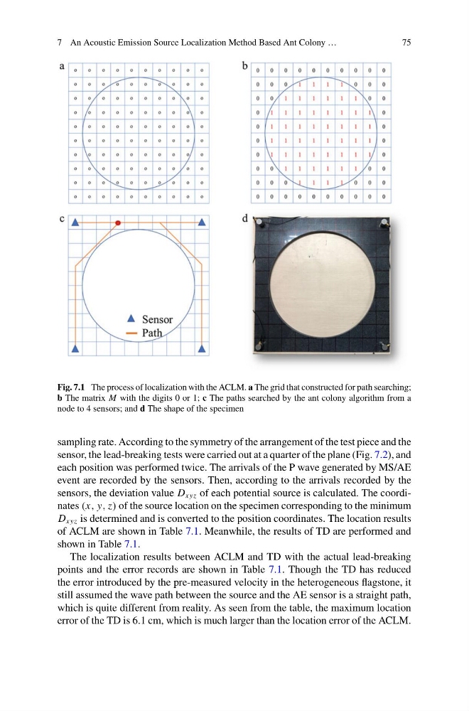
Fig. 7.1 The process of localization with the ACLM. a The grid that constructed for path searching;
b The matrix M with the digits 0 or 1; c The paths searched by the ant colony algorithm from a
node to 4 sensors; and d The shape of the specimen
sampling rate. According to the symmetry of the arrangement of the test piece and the
sensor, the lead-breaking tests were carried out at a quarter of the plane (Fig. 7.2), and
each position was performed twice. The arrivals of the P wave generated by MS/AE
event are recorded by the sensors. Then, according to the arrivals recorded by the
sensors, the deviation value D xyz of each potential source is calculated. The coordinates (x, y, z) of the source location on the specimen corresponding to the minimum
D xyz is determined and is converted to the position coordinates. The location results
of ACLM are shown in Table 7.1. Meanwhile, the results of TD are performed and
shown in Table 7.1.
The localization results between ACLM and TD with the actual lead-breaking
points and the error records are shown in Table 7.1. Though the TD has reduced
the error introduced by the pre-measured velocity in the heterogeneous flagstone, it
still assumed the wave path between the source and the AE sensor is a straight path,
which is quite different from reality. As seen from the table, the maximum location
error of the TD is 6.1 cm, which is much larger than the location error of the ACLM.
75
Fig. 7.1 The process of localization with the ACLM. a The grid that constructed for path searching;
b The matrix M with the digits 0 or 1; c The paths searched by the ant colony algorithm from a
node to 4 sensors; and d The shape of the specimen
sampling rate. According to the symmetry of the arrangement of the test piece and the
sensor, the lead-breaking tests were carried out at a quarter of the plane (Fig. 7.2), and
each position was performed twice. The arrivals of the P wave generated by MS/AE
event are recorded by the sensors. Then, according to the arrivals recorded by the
sensors, the deviation value D xyz of each potential source is calculated. The coordinates (x, y, z) of the source location on the specimen corresponding to the minimum
D xyz is determined and is converted to the position coordinates. The location results
of ACLM are shown in Table 7.1. Meanwhile, the results of TD are performed and
shown in Table 7.1.
The localization results between ACLM and TD with the actual lead-breaking
points and the error records are shown in Table 7.1. Though the TD has reduced
the error introduced by the pre-measured velocity in the heterogeneous flagstone, it
still assumed the wave path between the source and the AE sensor is a straight path,
which is quite different from reality. As seen from the table, the maximum location
error of the TD is 6.1 cm, which is much larger than the location error of the ACLM.