

74
Q. Hu and L. Dong
coordinates of AE source (x 0 , y 0 ), initial time of excitation t 0 ), so sensor number
m should be an integer greater than or equal to 4. For the kth sensor S k receiving
the signal, the coordinates are recorded as (x k , y k ), and the first arrival time of the
received P wave signal is t
k
0 . Calculate the actual time difference of the two different
sensors S l and S m , denoted by t
lm
0 .
7.2.6 Source Location
According to the square of the difference between t
lm
0 and t
lm
xy , D is introduced
to describe the deviation degree of the point P xyz from the unknown MS/AE source
P 0 , which is expressed as:
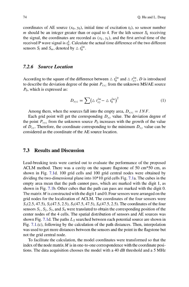
D xyz =
t
lm
xy − t
lm
0
2
(1)
Among them, when the sources fall into the empty area, D xyz = I N F.
Each grid point will get the corresponding D xy value. The deviation degree of
the point P xyz from the unknown source P 0 increases with the growth of the value
of D xy . Therefore, the coordinate corresponding to the minimum D xy value can be
considered as the coordinate of the AE source location.
7.3 Results and Discussion
Lead-breaking tests were carried out to evaluate the performance of the proposed
ACLM method. There was a cavity on the square flagstone of 50 cm*50 cm, as
shown in Fig. 7.1d. 100 grid cells and 100 grid central nodes were obtained by
dividing the two-dimensional plane into 10*10 grid cells Fig. 7.1a. The cubes in the
empty area mean that the path cannot pass, which are marked with the digit 1, as
shown in Fig. 7.1b. Other cubes that the path can pass are marked with the digit 0.
The matrix M is constructed with the digit 1 and 0. Four sensors were arranged on the
grid nodes for the localization of ACLM. The coordinates of the four sensors were
S 1 (2.5, 47.5), S 2 (47.5, 2.5), S 3 (47.5, 47.5), S 4 (47.5, 2.5). The coordinates of the four
sensors S 1 , S 2 , S 3 , and S 4 were translated to obtain the corresponding position of the
center nodes of the 4 cells. The spatial distribution of sensors and AE sources was
shown Fig. 7.1d. The paths L S searched between each potential source are shown in
Fig. 7.1.(c), following by the calculation of the path distances. Then, interpolation
was used to get more distances between the sensors and the point in the flagstone but
not the grid central node.
To facilitate the calculation, the model coordinates were transformed so that the
index of the node matrix M is in one-to-one correspondence with the coordinate positions. The data acquisition chooses the model with a 40 dB threshold and a 5 MHz
Q. Hu and L. Dong
coordinates of AE source (x 0 , y 0 ), initial time of excitation t 0 ), so sensor number
m should be an integer greater than or equal to 4. For the kth sensor S k receiving
the signal, the coordinates are recorded as (x k , y k ), and the first arrival time of the
received P wave signal is t
k
0 . Calculate the actual time difference of the two different
sensors S l and S m , denoted by t
lm
0 .
7.2.6 Source Location
According to the square of the difference between t
lm
0 and t
lm
xy , D is introduced
to describe the deviation degree of the point P xyz from the unknown MS/AE source
P 0 , which is expressed as:
D xyz =
t
lm
xy − t
lm
0
2
(1)
Among them, when the sources fall into the empty area, D xyz = I N F.
Each grid point will get the corresponding D xy value. The deviation degree of
the point P xyz from the unknown source P 0 increases with the growth of the value
of D xy . Therefore, the coordinate corresponding to the minimum D xy value can be
considered as the coordinate of the AE source location.
7.3 Results and Discussion
Lead-breaking tests were carried out to evaluate the performance of the proposed
ACLM method. There was a cavity on the square flagstone of 50 cm*50 cm, as
shown in Fig. 7.1d. 100 grid cells and 100 grid central nodes were obtained by
dividing the two-dimensional plane into 10*10 grid cells Fig. 7.1a. The cubes in the
empty area mean that the path cannot pass, which are marked with the digit 1, as
shown in Fig. 7.1b. Other cubes that the path can pass are marked with the digit 0.
The matrix M is constructed with the digit 1 and 0. Four sensors were arranged on the
grid nodes for the localization of ACLM. The coordinates of the four sensors were
S 1 (2.5, 47.5), S 2 (47.5, 2.5), S 3 (47.5, 47.5), S 4 (47.5, 2.5). The coordinates of the four
sensors S 1 , S 2 , S 3 , and S 4 were translated to obtain the corresponding position of the
center nodes of the 4 cells. The spatial distribution of sensors and AE sources was
shown Fig. 7.1d. The paths L S searched between each potential source are shown in
Fig. 7.1.(c), following by the calculation of the path distances. Then, interpolation
was used to get more distances between the sensors and the point in the flagstone but
not the grid central node.
To facilitate the calculation, the model coordinates were transformed so that the
index of the node matrix M is in one-to-one correspondence with the coordinate positions. The data acquisition chooses the model with a 40 dB threshold and a 5 MHz