

43 The Influence of Rod Waveguide on Acoustic Emission …
495
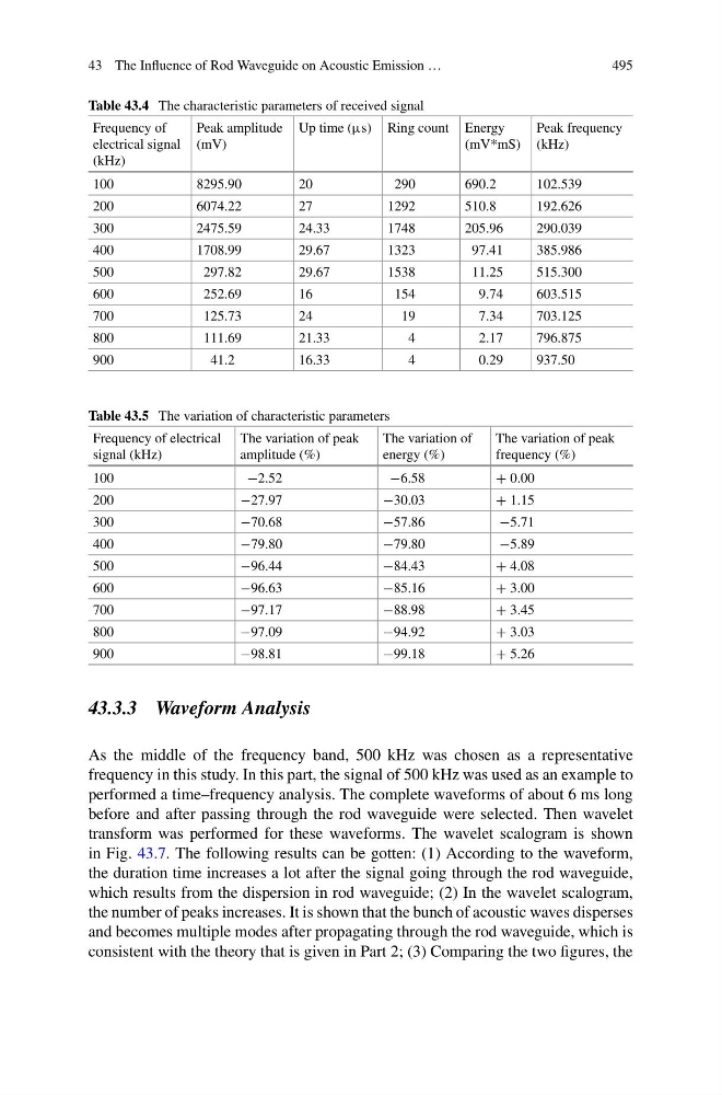
Table 43.4 The characteristic parameters of received signal
Frequency of
electrical signal
(kHz)
Peak amplitude
(mV)
Up time (µs) Ring count Energy
(mV*mS)
Peak frequency
(kHz)
100
8295.90
20
290
690.2
102.539
200
6074.22
27
1292
510.8
192.626
300
2475.59
24.33
1748
205.96
290.039
400
1708.99
29.67
1323
97.41
385.986
500
297.82
29.67
1538
11.25
515.300
600
252.69
16
154
9.74
603.515
700
125.73
24
19
7.34
703.125
800
111.69
21.33
4
2.17
796.875
900
41.2
16.33
4
0.29
937.50
Table 43.5 The variation of characteristic parameters
Frequency of electrical
signal (kHz)
The variation of peak
amplitude (%)
The variation of
energy (%)
The variation of peak
frequency (%)
100
−2.52
−6.58
+ 0.00
200
−27.97
−30.03
+ 1.15
300
−70.68
−57.86
−5.71
400
−79.80
−79.80
−5.89
500
−96.44
−84.43
+ 4.08
600
−96.63
−85.16
+ 3.00
700
−97.17
−88.98
+ 3.45
800
−97.09
−94.92
+ 3.03
900
−98.81
−99.18
+ 5.26
43.3.3 Waveform Analysis
As the middle of the frequency band, 500 kHz was chosen as a representative
frequency in this study. In this part, the signal of 500 kHz was used as an example to
performed a time–frequency analysis. The complete waveforms of about 6 ms long
before and after passing through the rod waveguide were selected. Then wavelet
transform was performed for these waveforms. The wavelet scalogram is shown
in Fig. 43.7. The following results can be gotten: (1) According to the waveform,
the duration time increases a lot after the signal going through the rod waveguide,
which results from the dispersion in rod waveguide; (2) In the wavelet scalogram,
the number of peaks increases. It is shown that the bunch of acoustic waves disperses
and becomes multiple modes after propagating through the rod waveguide, which is
consistent with the theory that is given in Part 2; (3) Comparing the two figures, the
495
Table 43.4 The characteristic parameters of received signal
Frequency of
electrical signal
(kHz)
Peak amplitude
(mV)
Up time (µs) Ring count Energy
(mV*mS)
Peak frequency
(kHz)
100
8295.90
20
290
690.2
102.539
200
6074.22
27
1292
510.8
192.626
300
2475.59
24.33
1748
205.96
290.039
400
1708.99
29.67
1323
97.41
385.986
500
297.82
29.67
1538
11.25
515.300
600
252.69
16
154
9.74
603.515
700
125.73
24
19
7.34
703.125
800
111.69
21.33
4
2.17
796.875
900
41.2
16.33
4
0.29
937.50
Table 43.5 The variation of characteristic parameters
Frequency of electrical
signal (kHz)
The variation of peak
amplitude (%)
The variation of
energy (%)
The variation of peak
frequency (%)
100
−2.52
−6.58
+ 0.00
200
−27.97
−30.03
+ 1.15
300
−70.68
−57.86
−5.71
400
−79.80
−79.80
−5.89
500
−96.44
−84.43
+ 4.08
600
−96.63
−85.16
+ 3.00
700
−97.17
−88.98
+ 3.45
800
−97.09
−94.92
+ 3.03
900
−98.81
−99.18
+ 5.26
43.3.3 Waveform Analysis
As the middle of the frequency band, 500 kHz was chosen as a representative
frequency in this study. In this part, the signal of 500 kHz was used as an example to
performed a time–frequency analysis. The complete waveforms of about 6 ms long
before and after passing through the rod waveguide were selected. Then wavelet
transform was performed for these waveforms. The wavelet scalogram is shown
in Fig. 43.7. The following results can be gotten: (1) According to the waveform,
the duration time increases a lot after the signal going through the rod waveguide,
which results from the dispersion in rod waveguide; (2) In the wavelet scalogram,
the number of peaks increases. It is shown that the bunch of acoustic waves disperses
and becomes multiple modes after propagating through the rod waveguide, which is
consistent with the theory that is given in Part 2; (3) Comparing the two figures, the