

31 Research on Immersion-Type Acoustic Emission …
367
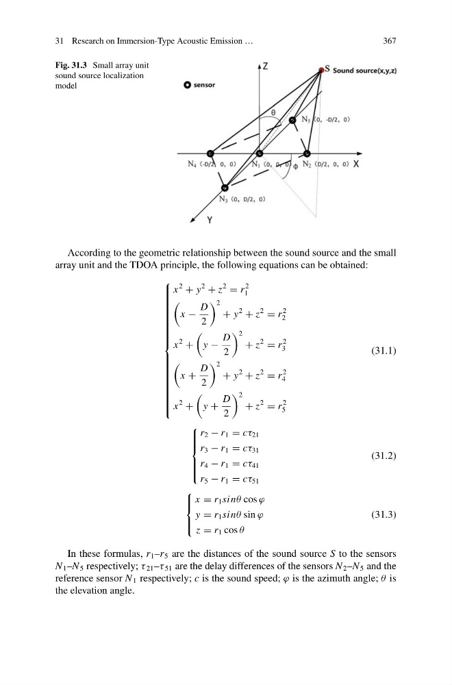
Fig. 31.3 Small array unit
sound source localization
model
According to the geometric relationship between the sound source and the small
array unit and the TDOA principle, the following equations can be obtained:
⎧
⎪ ⎪ ⎪ ⎪ ⎪ ⎪ ⎪ ⎪ ⎪ ⎪ ⎪ ⎪ ⎪ ⎪ ⎪ ⎪ ⎨
⎪ ⎪ ⎪ ⎪ ⎪ ⎪ ⎪ ⎪ ⎪ ⎪ ⎪ ⎪ ⎪ ⎪ ⎪ ⎪ ⎩
x
2
+ y
2
+ z
2
= r
2
1
x −
D
2
2
+ y
2
+ z
2
= r
2
2
x
2
+
y −
D
2
2
+ z
2
= r
2
3
x +
D
2
2
+ y
2
+ z
2
= r
2
4
x
2
+
y +
D
2
2
+ z
2
= r
2
5
(31.1)
⎧
⎪ ⎪ ⎪ ⎨
⎪ ⎪ ⎪ ⎩
r 2 − r 1 = cτ 21
r 3 − r 1 = cτ 31
r 4 − r 1 = cτ 41
r 5 − r 1 = cτ 51
(31.2)
⎧
⎪ ⎨
⎪ ⎩
x = r 1 sinθ cos ϕ
y = r 1 sinθ sin ϕ
z = r 1 cos θ
(31.3)
In these formulas, r 1 –r 5 are the distances of the sound source S to the sensors
N 1 –N 5 respectively; τ 21 –τ 51 are the delay differences of the sensors N 2 –N 5 and the
reference sensor N 1 respectively; c is the sound speed; ϕ is the azimuth angle; θ is
the elevation angle.
367
Fig. 31.3 Small array unit
sound source localization
model
According to the geometric relationship between the sound source and the small
array unit and the TDOA principle, the following equations can be obtained:
⎧
⎪ ⎪ ⎪ ⎪ ⎪ ⎪ ⎪ ⎪ ⎪ ⎪ ⎪ ⎪ ⎪ ⎪ ⎪ ⎪ ⎨
⎪ ⎪ ⎪ ⎪ ⎪ ⎪ ⎪ ⎪ ⎪ ⎪ ⎪ ⎪ ⎪ ⎪ ⎪ ⎪ ⎩
x
2
+ y
2
+ z
2
= r
2
1
x −
D
2
2
+ y
2
+ z
2
= r
2
2
x
2
+
y −
D
2
2
+ z
2
= r
2
3
x +
D
2
2
+ y
2
+ z
2
= r
2
4
x
2
+
y +
D
2
2
+ z
2
= r
2
5
(31.1)
⎧
⎪ ⎪ ⎪ ⎨
⎪ ⎪ ⎪ ⎩
r 2 − r 1 = cτ 21
r 3 − r 1 = cτ 31
r 4 − r 1 = cτ 41
r 5 − r 1 = cτ 51
(31.2)
⎧
⎪ ⎨
⎪ ⎩
x = r 1 sinθ cos ϕ
y = r 1 sinθ sin ϕ
z = r 1 cos θ
(31.3)
In these formulas, r 1 –r 5 are the distances of the sound source S to the sensors
N 1 –N 5 respectively; τ 21 –τ 51 are the delay differences of the sensors N 2 –N 5 and the
reference sensor N 1 respectively; c is the sound speed; ϕ is the azimuth angle; θ is
the elevation angle.