

26 Damage Evaluation Inside the Concrete Dam …
315
Meanwhile, as shown in Fig. 26.1, the target area is divided into several elements
and the “slowness”, which means the inverse of the velocity, is given into each
element as an initial parameter.
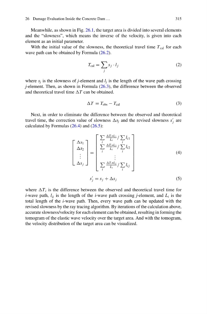
With the initial value of the slowness, the theoretical travel time T cal for each
wave path can be obtained by Formula (26.2).
T cal =
j
s j · l j
(2)
where s j is the slowness of j-element and l j is the length of the wave path crossing
j-element. Then, as shown in Formula (26.3), the difference between the observed
and theoretical travel time T can be obtained.
T = T obs − T cal
(3)
Next, in order to eliminate the difference between the observed and theoretical
travel time, the correction value of slowness s j and the revised slowness s
j are
calculated by Formulas (26.4) and (26.5):
⎡
⎢
⎢
⎢
⎣
s 1
s 2
. . .
s j
⎤
⎥
⎥
⎥
⎦
=
⎡
⎢
⎢
⎢
⎢
⎢
⎢
⎢
⎣
i
T i ∗l i1
L i
/
i
l i1
i
T i ∗l i2
L i
/
i
l i2
. . .
i
T i ∗l i j
L i
/
i
l i j
⎤
⎥
⎥
⎥
⎥
⎥
⎥
⎥
⎦
(4)
s
j = s j + s j
(5)
where T i is the difference between the observed and theoretical travel time for
i-wave path, l ij is the length of the i-wave path crossing j-element, and L i is the
total length of the i-wave path. Then, every wave path can be updated with the
revised slowness by the ray tracing algorithm. By iterations of the calculation above,
accurate slowness/velocity for each element can be obtained, resulting in forming the
tomogram of the elastic wave velocity over the target area. And with the tomogram,
the velocity distribution of the target area can be visualized.
315
Meanwhile, as shown in Fig. 26.1, the target area is divided into several elements
and the “slowness”, which means the inverse of the velocity, is given into each
element as an initial parameter.
With the initial value of the slowness, the theoretical travel time T cal for each
wave path can be obtained by Formula (26.2).
T cal =
j
s j · l j
(2)
where s j is the slowness of j-element and l j is the length of the wave path crossing
j-element. Then, as shown in Formula (26.3), the difference between the observed
and theoretical travel time T can be obtained.
T = T obs − T cal
(3)
Next, in order to eliminate the difference between the observed and theoretical
travel time, the correction value of slowness s j and the revised slowness s
j are
calculated by Formulas (26.4) and (26.5):
⎡
⎢
⎢
⎢
⎣
s 1
s 2
. . .
s j
⎤
⎥
⎥
⎥
⎦
=
⎡
⎢
⎢
⎢
⎢
⎢
⎢
⎢
⎣
i
T i ∗l i1
L i
/
i
l i1
i
T i ∗l i2
L i
/
i
l i2
. . .
i
T i ∗l i j
L i
/
i
l i j
⎤
⎥
⎥
⎥
⎥
⎥
⎥
⎥
⎦
(4)
s
j = s j + s j
(5)
where T i is the difference between the observed and theoretical travel time for
i-wave path, l ij is the length of the i-wave path crossing j-element, and L i is the
total length of the i-wave path. Then, every wave path can be updated with the
revised slowness by the ray tracing algorithm. By iterations of the calculation above,
accurate slowness/velocity for each element can be obtained, resulting in forming the
tomogram of the elastic wave velocity over the target area. And with the tomogram,
the velocity distribution of the target area can be visualized.