

178
S. Wu et al.
Time/s
(a) the first IMF component
Time/s
(b) the second IMF component
Time/s
(c) the third IMF component
Time/s
(d) the fourth IMF component
Time/s
(f) the sixth IMF component
Time/s
(e) the fifthIMFcomponent
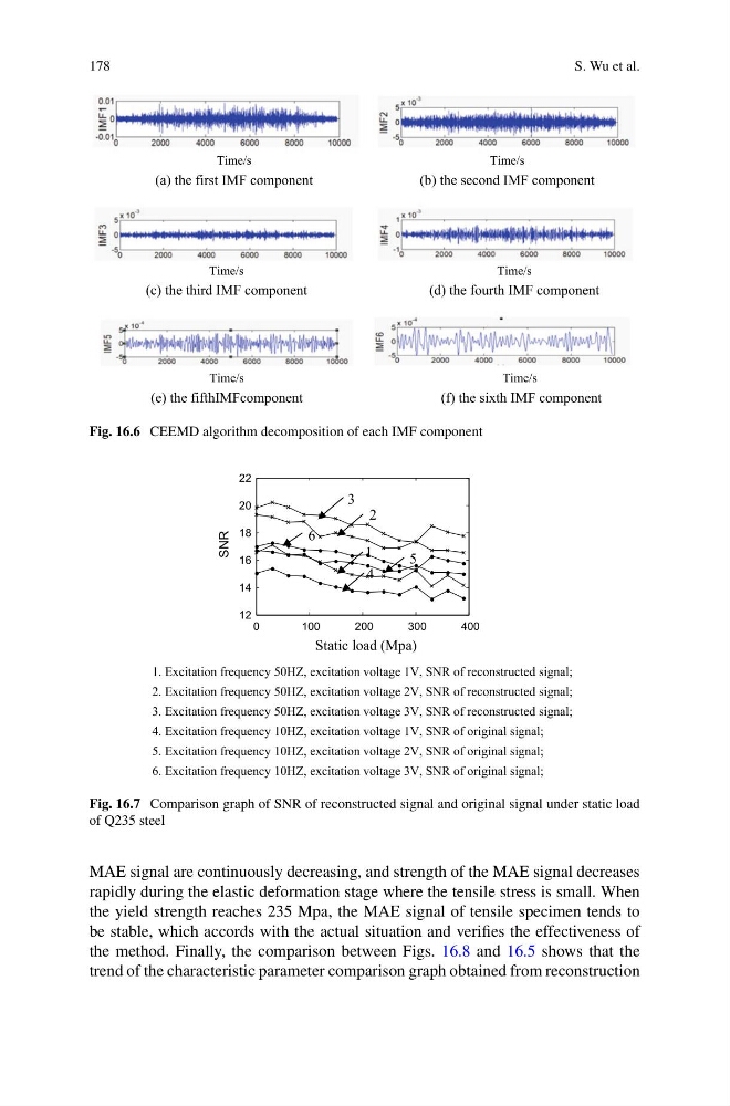
Fig. 16.6 CEEMD algorithm decomposition of each IMF component
0
100
200
300
400
12
14
16
18
20
22
SNR
1
2
3
4
5
6
Static load (Mpa)
1. Excitation frequency 50HZ, excitation voltage 1V, SNR of reconstructed signal;
2. Excitation frequency 50HZ, excitation voltage 2V, SNR of reconstructed signal;
3. Excitation frequency 50HZ, excitation voltage 3V, SNR of reconstructed signal;
4. Excitation frequency 10HZ, excitation voltage 1V, SNR of original signal;
5. Excitation frequency 10HZ, excitation voltage 2V, SNR of original signal;
6. Excitation frequency 10HZ, excitation voltage 3V, SNR of original signal;
Fig. 16.7 Comparison graph of SNR of reconstructed signal and original signal under static load
of Q235 steel
MAE signal are continuously decreasing, and strength of the MAE signal decreases
rapidly during the elastic deformation stage where the tensile stress is small. When
the yield strength reaches 235 Mpa, the MAE signal of tensile specimen tends to
be stable, which accords with the actual situation and verifies the effectiveness of
the method. Finally, the comparison between Figs. 16.8 and 16.5 shows that the
trend of the characteristic parameter comparison graph obtained from reconstruction
S. Wu et al.
Time/s
(a) the first IMF component
Time/s
(b) the second IMF component
Time/s
(c) the third IMF component
Time/s
(d) the fourth IMF component
Time/s
(f) the sixth IMF component
Time/s
(e) the fifthIMFcomponent
Fig. 16.6 CEEMD algorithm decomposition of each IMF component
0
100
200
300
400
12
14
16
18
20
22
SNR
1
2
3
4
5
6
Static load (Mpa)
1. Excitation frequency 50HZ, excitation voltage 1V, SNR of reconstructed signal;
2. Excitation frequency 50HZ, excitation voltage 2V, SNR of reconstructed signal;
3. Excitation frequency 50HZ, excitation voltage 3V, SNR of reconstructed signal;
4. Excitation frequency 10HZ, excitation voltage 1V, SNR of original signal;
5. Excitation frequency 10HZ, excitation voltage 2V, SNR of original signal;
6. Excitation frequency 10HZ, excitation voltage 3V, SNR of original signal;
Fig. 16.7 Comparison graph of SNR of reconstructed signal and original signal under static load
of Q235 steel
MAE signal are continuously decreasing, and strength of the MAE signal decreases
rapidly during the elastic deformation stage where the tensile stress is small. When
the yield strength reaches 235 Mpa, the MAE signal of tensile specimen tends to
be stable, which accords with the actual situation and verifies the effectiveness of
the method. Finally, the comparison between Figs. 16.8 and 16.5 shows that the
trend of the characteristic parameter comparison graph obtained from reconstruction