

98
B. P. Duong et al.
in this sample. If the hypothesis (H 1 ) is more appropriate, the detection algorithm
affirms that the object is present. Assume the process is applied to a one-dimension
signal (1 × m) sample. This signal is segmented by windowing to n segments. Each
segment is associated with a test cell (C T ) and contains N samples. ECFAR calculates the detection threshold depends on the power in the cells which surround the
test cell. The immediate cells next to the test cell are called neighbor cells. These
neighbor cells are excluded from the average calculation to detect if the object is
presented. Because of the fact that bursts, or impulses, are not located at one cell but
rather spreads across some range cells, the reference segment is not directly placed
nearby the test cell. An adaptive threshold (T ) is estimated depending on values from
the surrounding cells of this test cell and a multiplier coefficient (α). This multiplier
coefficient is a constant that is determined to associate with the false alarm probability
(P f a ) to attenuate or amplify the detection threshold. Hence, the ECFAR algorithm
maintains a constant false alarm rate but it makes varying in the detection threshold.
This indicates that contextual information around the test cell is considered in the
estimation of the threshold. This turns ECFAR into an adaptive method to make the
detections based on contextual information. Then, the comparison unit compares the
current test cell value with the detection threshold T . If the test cell value exceeds the
threshold, the algorithm affirms that the object is present. This process is recursively
employed in the next cell.
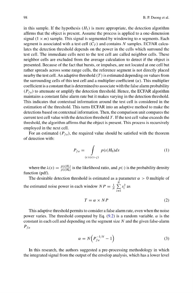
For an estimated (P f a ), the required value should be satisfied with the theorem
of detection with:
P f a =
(s:λ(s)>ς)
p(s|H 0 )ds
(1)
where the λ(s) =
p(s|H 1 )
p(s|H 0 )
is the likelihood ratio, and p(·) is the probability density
function (pdf).
The desirable detection threshold is estimated as a parameter α > 0 multiple of
the estimated noise power in each window N P =
1
N
N
i=1
s
2
i as
T = α × N P
(2)
This adaptive threshold permits to consider a false alarm rate, even when the noise
power varies. The threshold computed by Eq. (9.2) is a random variable. α is the
constant in each cell and depending on the segment size N and the given false-alarm
P f a
α = N
P
−1/N
f a
− 1
(3)
In this research, the authors suggested a pre-processing methodology in which
the integrated signal from the output of the envelop analysis, which has a lower level
B. P. Duong et al.
in this sample. If the hypothesis (H 1 ) is more appropriate, the detection algorithm
affirms that the object is present. Assume the process is applied to a one-dimension
signal (1 × m) sample. This signal is segmented by windowing to n segments. Each
segment is associated with a test cell (C T ) and contains N samples. ECFAR calculates the detection threshold depends on the power in the cells which surround the
test cell. The immediate cells next to the test cell are called neighbor cells. These
neighbor cells are excluded from the average calculation to detect if the object is
presented. Because of the fact that bursts, or impulses, are not located at one cell but
rather spreads across some range cells, the reference segment is not directly placed
nearby the test cell. An adaptive threshold (T ) is estimated depending on values from
the surrounding cells of this test cell and a multiplier coefficient (α). This multiplier
coefficient is a constant that is determined to associate with the false alarm probability
(P f a ) to attenuate or amplify the detection threshold. Hence, the ECFAR algorithm
maintains a constant false alarm rate but it makes varying in the detection threshold.
This indicates that contextual information around the test cell is considered in the
estimation of the threshold. This turns ECFAR into an adaptive method to make the
detections based on contextual information. Then, the comparison unit compares the
current test cell value with the detection threshold T . If the test cell value exceeds the
threshold, the algorithm affirms that the object is present. This process is recursively
employed in the next cell.
For an estimated (P f a ), the required value should be satisfied with the theorem
of detection with:
P f a =
(s:λ(s)>ς)
p(s|H 0 )ds
(1)
where the λ(s) =
p(s|H 1 )
p(s|H 0 )
is the likelihood ratio, and p(·) is the probability density
function (pdf).
The desirable detection threshold is estimated as a parameter α > 0 multiple of
the estimated noise power in each window N P =
1
N
N
i=1
s
2
i as
T = α × N P
(2)
This adaptive threshold permits to consider a false alarm rate, even when the noise
power varies. The threshold computed by Eq. (9.2) is a random variable. α is the
constant in each cell and depending on the segment size N and the given false-alarm
P f a
α = N
P
−1/N
f a
− 1
(3)
In this research, the authors suggested a pre-processing methodology in which
the integrated signal from the output of the envelop analysis, which has a lower level