

K.2 One-Dimensional Hydrogen
533
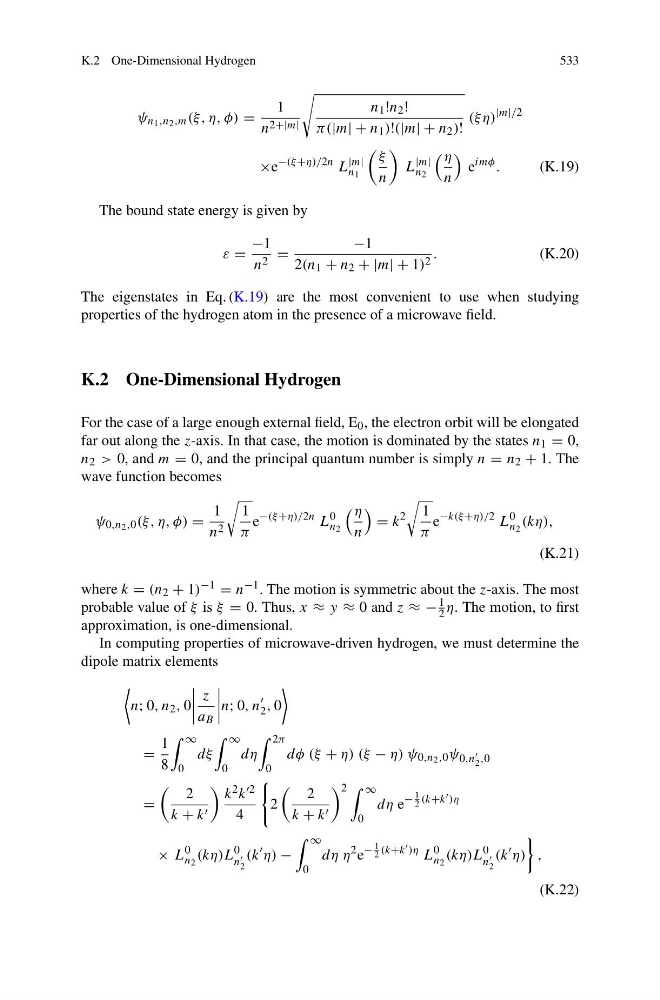
ψ n 1 ,n 2 ,m (ξ, η, φ) =
1
n 2+|m|
n 1 !n 2 !
π(|m| + n 1 )!(|m| + n 2 )!
(ξ η)
|m|/2
×e
−(ξ +η)/2n L
|m|
n 1
ξ
n
L
|m|
n 2
η
n
e
imφ .
(K.19)
The bound state energy is given by
ε =
−1
n 2 =
−1
2(n 1 + n 2 + |m| + 1) 2 .
(K.20)
The eigenstates in Eq. (K.19) are the most convenient to use when studying
properties of the hydrogen atom in the presence of a microwave field.
K.2 One-Dimensional Hydrogen
For the case of a large enough external field, E 0 , the electron orbit will be elongated
far out along the z-axis. In that case, the motion is dominated by the states n 1 = 0,
n 2 > 0, and m = 0, and the principal quantum number is simply n = n 2 + 1. The
wave function becomes
ψ 0,n 2 ,0 (ξ, η, φ) =
1
n 2
1
π
e
−(ξ +η)/2n L
0
n 2
η
n
= k
2
1
π
e
−k(ξ +η)/2 L
0
n 2
(kη),
(K.21)
where k = (n 2 + 1) −1 = n −1 . The motion is symmetric about the z-axis. The most
probable value of ξ is ξ = 0. Thus, x ≈ y ≈ 0 and z ≈ −
1
2 η. The motion, to first
approximation, is one-dimensional.
In computing properties of microwave-driven hydrogen, we must determine the
dipole matrix elements
n; 0, n 2 , 0
z
a B
n; 0, n
2 , 0
=
1
8
∞
0
dξ
∞
0
dη
2π
0
dφ (ξ + η) (ξ − η) ψ 0,n 2 ,0 ψ 0,n
2 ,0
=
2
k + k
k 2 k 2
4
2
2
k + k
2 ∞
0
dη e
−
1
2 (k+k )η
× L
0
n 2
(kη)L
0
n
2
(k
η) −
∞
0
dη η
2 e
−
1
2 (k+k )η L
0
n 2
(kη)L
0
n
2
(k
η)
,
(K.22)
533
ψ n 1 ,n 2 ,m (ξ, η, φ) =
1
n 2+|m|
n 1 !n 2 !
π(|m| + n 1 )!(|m| + n 2 )!
(ξ η)
|m|/2
×e
−(ξ +η)/2n L
|m|
n 1
ξ
n
L
|m|
n 2
η
n
e
imφ .
(K.19)
The bound state energy is given by
ε =
−1
n 2 =
−1
2(n 1 + n 2 + |m| + 1) 2 .
(K.20)
The eigenstates in Eq. (K.19) are the most convenient to use when studying
properties of the hydrogen atom in the presence of a microwave field.
K.2 One-Dimensional Hydrogen
For the case of a large enough external field, E 0 , the electron orbit will be elongated
far out along the z-axis. In that case, the motion is dominated by the states n 1 = 0,
n 2 > 0, and m = 0, and the principal quantum number is simply n = n 2 + 1. The
wave function becomes
ψ 0,n 2 ,0 (ξ, η, φ) =
1
n 2
1
π
e
−(ξ +η)/2n L
0
n 2
η
n
= k
2
1
π
e
−k(ξ +η)/2 L
0
n 2
(kη),
(K.21)
where k = (n 2 + 1) −1 = n −1 . The motion is symmetric about the z-axis. The most
probable value of ξ is ξ = 0. Thus, x ≈ y ≈ 0 and z ≈ −
1
2 η. The motion, to first
approximation, is one-dimensional.
In computing properties of microwave-driven hydrogen, we must determine the
dipole matrix elements
n; 0, n 2 , 0
z
a B
n; 0, n
2 , 0
=
1
8
∞
0
dξ
∞
0
dη
2π
0
dφ (ξ + η) (ξ − η) ψ 0,n 2 ,0 ψ 0,n
2 ,0
=
2
k + k
k 2 k 2
4
2
2
k + k
2 ∞
0
dη e
−
1
2 (k+k )η
× L
0
n 2
(kη)L
0
n
2
(k
η) −
∞
0
dη η
2 e
−
1
2 (k+k )η L
0
n 2
(kη)L
0
n
2
(k
η)
,
(K.22)