

534
K Hydrogen in a Constant Electric Field
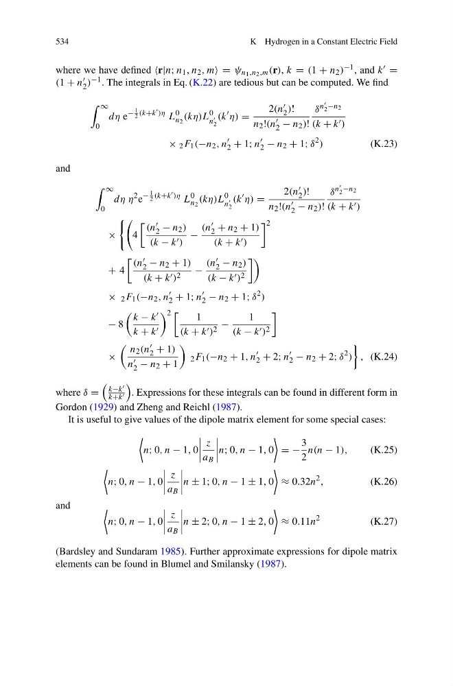
where we have defined r|n; n 1 , n 2 , m = ψ n 1 ,n 2 ,m (r), k = (1 + n 2 ) −1 , and k =
(1 + n
2 ) −1 . The integrals in Eq. (K.22) are tedious but can be computed. We find
∞
0
dη e
−
1
2 (k+k )η L
0
n 2
(kη)L
0
n
2
(k
η) =
2(n
2 )!
n 2 !(n
2 − n 2 )!
δ
n
2 −n 2
(k + k )
× 2 F 1 (−n 2 , n
2 + 1; n
2 − n 2 + 1; δ
2 )
(K.23)
and
∞
0
dη η
2 e
−
1
2 (k+k )η L
0
n 2
(kη)L
0
n
2
(k
η) =
2(n
2 )!
n 2 !(n
2 − n 2 )!
δ
n
2 −n 2
(k + k )
×
4
(n
2 − n 2 )
(k − k )
−
(n
2 + n 2 + 1)
(k + k )
2
+ 4
(n
2 − n 2 + 1)
(k + k ) 2 −
(n
2 − n 2 )
(k − k ) 2
× 2 F 1 (−n 2 , n
2 + 1; n
2 − n 2 + 1; δ
2 )
− 8
k − k
k + k
2
1
(k + k ) 2 −
1
(k − k ) 2
×
n 2 (n
2 + 1)
n
2 − n 2 + 1
2 F 1 (−n 2 + 1, n
2 + 2; n
2 − n 2 + 2; δ
2 )
, (K.24)
where δ =
k−k
k+k
. Expressions for these integrals can be found in different form in
Gordon (1929) and Zheng and Reichl (1987).
It is useful to give values of the dipole matrix element for some special cases:
n; 0, n − 1, 0
z
a B
n; 0, n − 1, 0
= −
3
2
n(n − 1),
(K.25)
n; 0, n − 1, 0
z
a B
n ± 1; 0, n − 1 ± 1, 0
≈ 0.32n
2 ,
(K.26)
and
n; 0, n − 1, 0
z
a B
n ± 2; 0, n − 1 ± 2, 0
≈ 0.11n
2
(K.27)
(Bardsley and Sundaram 1985). Further approximate expressions for dipole matrix
elements can be found in Blumel and Smilansky (1987).
K Hydrogen in a Constant Electric Field
where we have defined r|n; n 1 , n 2 , m = ψ n 1 ,n 2 ,m (r), k = (1 + n 2 ) −1 , and k =
(1 + n
2 ) −1 . The integrals in Eq. (K.22) are tedious but can be computed. We find
∞
0
dη e
−
1
2 (k+k )η L
0
n 2
(kη)L
0
n
2
(k
η) =
2(n
2 )!
n 2 !(n
2 − n 2 )!
δ
n
2 −n 2
(k + k )
× 2 F 1 (−n 2 , n
2 + 1; n
2 − n 2 + 1; δ
2 )
(K.23)
and
∞
0
dη η
2 e
−
1
2 (k+k )η L
0
n 2
(kη)L
0
n
2
(k
η) =
2(n
2 )!
n 2 !(n
2 − n 2 )!
δ
n
2 −n 2
(k + k )
×
4
(n
2 − n 2 )
(k − k )
−
(n
2 + n 2 + 1)
(k + k )
2
+ 4
(n
2 − n 2 + 1)
(k + k ) 2 −
(n
2 − n 2 )
(k − k ) 2
× 2 F 1 (−n 2 , n
2 + 1; n
2 − n 2 + 1; δ
2 )
− 8
k − k
k + k
2
1
(k + k ) 2 −
1
(k − k ) 2
×
n 2 (n
2 + 1)
n
2 − n 2 + 1
2 F 1 (−n 2 + 1, n
2 + 2; n
2 − n 2 + 2; δ
2 )
, (K.24)
where δ =
k−k
k+k
. Expressions for these integrals can be found in different form in
Gordon (1929) and Zheng and Reichl (1987).
It is useful to give values of the dipole matrix element for some special cases:
n; 0, n − 1, 0
z
a B
n; 0, n − 1, 0
= −
3
2
n(n − 1),
(K.25)
n; 0, n − 1, 0
z
a B
n ± 1; 0, n − 1 ± 1, 0
≈ 0.32n
2 ,
(K.26)
and
n; 0, n − 1, 0
z
a B
n ± 2; 0, n − 1 ± 2, 0
≈ 0.11n
2
(K.27)
(Bardsley and Sundaram 1985). Further approximate expressions for dipole matrix
elements can be found in Blumel and Smilansky (1987).