496
G Circular Ensembles
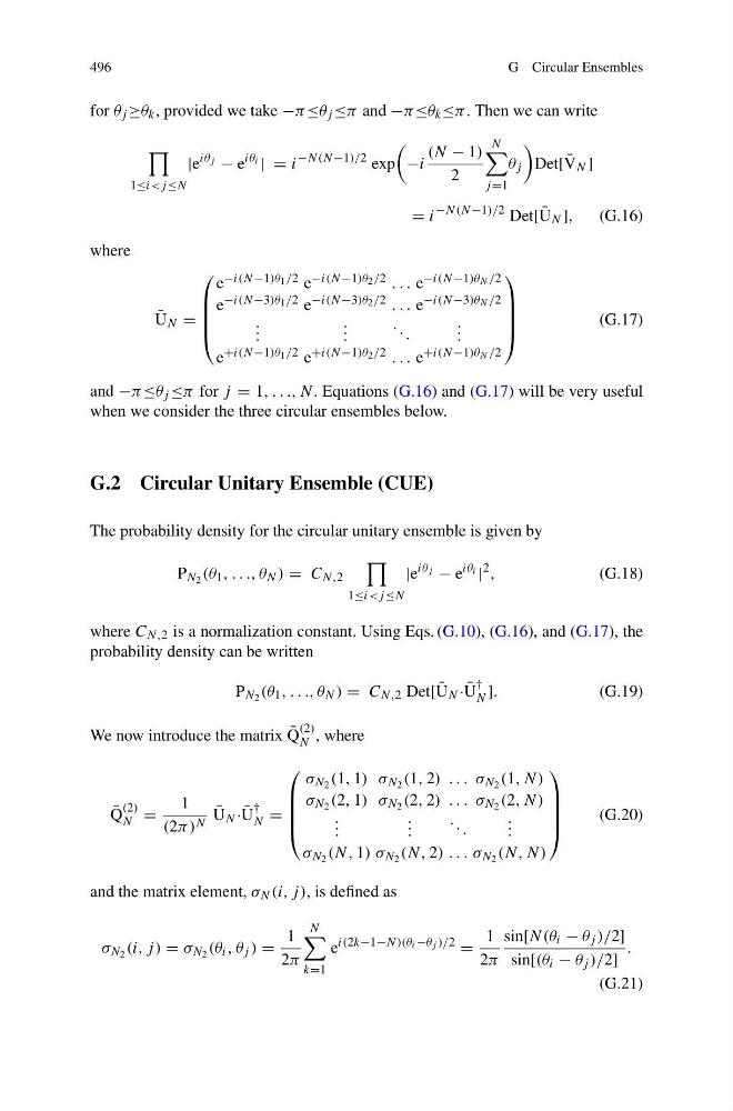
for θ j ≥θ k , provided we take −π ≤θ j ≤π and −π ≤θ k ≤π . Then we can write
1≤i |e
iθ j − e
iθ i | = i
−N(N−1)/2 exp
−i
(N − 1)
2
N
j =1
θ j
Det[ ¯
V N ]
= i
−N(N−1)/2 Det[ ¯
U N ],
(G.16)
where
¯
U N =
⎛
⎜
⎜
⎜
⎝
e −i(N−1)θ 1 /2 e −i(N−1)θ 2 /2 . . . e −i(N−1)θ N /2
e −i(N−3)θ 1 /2 e −i(N−3)θ 2 /2 . . . e −i(N−3)θ N /2
. . .
. . .
. . .
. . .
e +i(N−1)θ 1 /2 e +i(N−1)θ 2 /2 . . . e +i(N−1)θ N /2
⎞
⎟
⎟
⎟
⎠
(G.17)
and −π ≤θ j ≤π for j = 1, . . ., N. Equations (G.16) and (G.17) will be very useful
when we consider the three circular ensembles below.
G.2 Circular Unitary Ensemble (CUE)
The probability density for the circular unitary ensemble is given by
P N 2 (θ 1 , . . ., θ N ) = C N,2
1≤i |e
iθ j − e
iθ i |
2 ,
(G.18)
where C N,2 is a normalization constant. Using Eqs. (G.10), (G.16), and (G.17), the
probability density can be written
P N 2 (θ 1 , . . ., θ N ) = C N,2 Det[ ¯
U N · ¯
U
†
N ].
(G.19)
We now introduce the matrix ¯
Q
(2)
N , where
¯
Q
(2)
N =
1
(2π) N
¯
U N · ¯
U
†
N =
⎛
⎜
⎜
⎜
⎝
σ N 2 (1, 1) σ N 2 (1, 2) . . . σ N 2 (1, N)
σ N 2 (2, 1) σ N 2 (2, 2) . . . σ N 2 (2, N)
. . .
. . .
. . .
. . .
σ N 2 (N, 1) σ N 2 (N, 2) . . . σ N 2 (N, N)
⎞
⎟
⎟
⎟
⎠
(G.20)
and the matrix element, σ N (i, j ), is defined as
σ N 2 (i, j ) = σ N 2 (θ i , θ j ) =
1
2π
N
k=1
e
i(2k−1−N )(θ i −θ j )/2
=
1
2π
sin[N(θ i − θ j )/2]
sin[(θ i − θ j )/2]
.
(G.21)