

386
10 Time-Periodic Quantum Systems
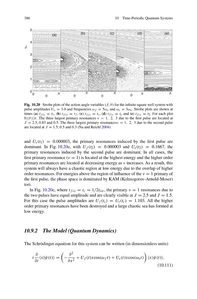
Fig. 10.20 Strobe plots of the action-angle variables (J, θ) for the infinite square well system with
pulse amplitudes U o = 3.0 and frequencies ω f = 5ω o and ω s = 3ω o . Strobe plots are shown at
times (a) t f ix = t 1 , (b) t f ix = t f , (c) t f ix = t c , (d) t f ix = t s and (e) t f ix = t 2 . For each plot
0≤θ≤π . The three largest primary resonances ν = 1, 2, 3 due to the first pulse are located at
J = 2.5, 0.83 and 0.5. The three largest primary resonancesν = 1, 2, 3 due to the second pulse
are located at J = 1.5, 0.5 and 0.3 (Na and Reichl 2004)
and U s (t 1 ) = 0.000003, the primary resonances induced by the first pulse are
dominant. In Fig. 10.20e, with U f (t 2 ) = 0.000003 and U s (t 2 ) = 0.1667, the
primary resonances induced by the second pulse are dominant. In all cases, the
first primary resonance (ν = 1) is located at the highest energy and the higher order
primary resonances are located at decreasing energy as ν increases. As a result, this
system will always have a chaotic region at low energy due to the overlap of higher
order resonances. For energies above the region of influence of the ν = 1 primary of
the first pulse, the phase space is dominated by KAM (Kolmogorov-Arnold-Moser)
tori.
In Fig. 10.20c, where t f ix = t c = 1/2t tot , the primary ν = 1 resonances due to
the two pulses have equal amplitude and are clearly visible at J = 2.5 and J = 1.5.
For this case the pulse amplitudes are U f (t c ) = U s (t c ) = 1.103. All the higher
order primary resonances have been destroyed and a large chaotic sea has formed at
low energy.
10.9.2 The Model (Quantum Dynamics)
The Schrödinger equation for this system can be written (in dimensionless units)
i
∂
∂t
=
−
∂ 2
∂x 2 + U f (t)xcos(ω f t) + U s (t)xcos(ω s t)
(10.111)
10 Time-Periodic Quantum Systems
Fig. 10.20 Strobe plots of the action-angle variables (J, θ) for the infinite square well system with
pulse amplitudes U o = 3.0 and frequencies ω f = 5ω o and ω s = 3ω o . Strobe plots are shown at
times (a) t f ix = t 1 , (b) t f ix = t f , (c) t f ix = t c , (d) t f ix = t s and (e) t f ix = t 2 . For each plot
0≤θ≤π . The three largest primary resonances ν = 1, 2, 3 due to the first pulse are located at
J = 2.5, 0.83 and 0.5. The three largest primary resonancesν = 1, 2, 3 due to the second pulse
are located at J = 1.5, 0.5 and 0.3 (Na and Reichl 2004)
and U s (t 1 ) = 0.000003, the primary resonances induced by the first pulse are
dominant. In Fig. 10.20e, with U f (t 2 ) = 0.000003 and U s (t 2 ) = 0.1667, the
primary resonances induced by the second pulse are dominant. In all cases, the
first primary resonance (ν = 1) is located at the highest energy and the higher order
primary resonances are located at decreasing energy as ν increases. As a result, this
system will always have a chaotic region at low energy due to the overlap of higher
order resonances. For energies above the region of influence of the ν = 1 primary of
the first pulse, the phase space is dominated by KAM (Kolmogorov-Arnold-Moser)
tori.
In Fig. 10.20c, where t f ix = t c = 1/2t tot , the primary ν = 1 resonances due to
the two pulses have equal amplitude and are clearly visible at J = 2.5 and J = 1.5.
For this case the pulse amplitudes are U f (t c ) = U s (t c ) = 1.103. All the higher
order primary resonances have been destroyed and a large chaotic sea has formed at
low energy.
10.9.2 The Model (Quantum Dynamics)
The Schrödinger equation for this system can be written (in dimensionless units)
i
∂
∂t
=
−
∂ 2
∂x 2 + U f (t)xcos(ω f t) + U s (t)xcos(ω s t)
(10.111)