

10.9 Quantum Control
385
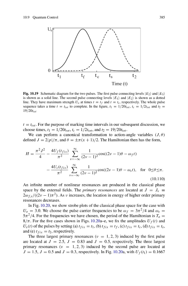
Fig. 10.19 Schematic diagram for the two pulses. The first pulse connecting levels |E 2 and |E 3
is shown as a solid line. The second pulse connecting levels |E 1 and |E 2 is shown as a dotted
line. They have maximum strength U o at times t = t f and t = t s , respectively. The whole pulse
sequence takes a time t = t tot to complete. In the figure, t 1 = 1/20t tot , t c = 1/2t tot and t 2 =
19/20t tot
t = t tot . For the purpose of marking time intervals in our subsequent discussion, we
choose times, t 1 = 1/20t tot , t c = 1/2t tot , and t 2 = 19/20t tot .
We can perform a canonical transformation to action-angle variables (J, θ )
defined J = 2|p|/π , and θ = ±π(x + 1)/2. The Hamiltonian then has the form,
H =
π 2 J 2
4
−
4U f (t f ix )
π 2
∞
ν=−∞
1
(2ν − 1) 2 cos((2ν − 1)θ − ω f t)
−
4U s (t f ix )
π 2
∞
ν=−∞
1
(2ν − 1) 2 cos((2ν − 1)θ − ω s t), for 0≤θ ≤π.
(10.110)
An infinite number of nonlinear resonances are produced in the classical phase
space by the external fields. The primary resonances are located at J = J ν ≡
2ω f,s /((2ν − 1)π 2 ). As ν increases, the location in energy of higher order primary
resonances decreases.
In Fig. 10.20, we show strobe plots of the classical phase space for the case with
U o = 3.0. We choose the pulse carrier frequencies to be ω f = 3π 2 /4 and ω s =
5π 2 /4. For the frequencies we have chosen, the period of the Hamiltonian is T o =
8/π . For the five cases shown in Figs. 10.20a–e, we fix the amplitudes U f (t) and
U s (t) of the pulses by setting (a) t f ix = t 1 , (b) t f ix = t f , (c) t f ix = t c , (d) t f ix = t s ,
and (e) t f ix = t 2 , respectively.
The three largest primary resonances (ν = 1, 2, 3) induced by the first pulse
are located at J = 2.5, J = 0.83 and J = 0.5, respectively. The three largest
primary resonances (ν = 1, 2, 3) induced by the second pulse are located at
J = 1.5, J = 0.5 and J = 0.3, respectively. In Fig. 10.20a, with U f (t 1 ) = 0.1667
385
Fig. 10.19 Schematic diagram for the two pulses. The first pulse connecting levels |E 2 and |E 3
is shown as a solid line. The second pulse connecting levels |E 1 and |E 2 is shown as a dotted
line. They have maximum strength U o at times t = t f and t = t s , respectively. The whole pulse
sequence takes a time t = t tot to complete. In the figure, t 1 = 1/20t tot , t c = 1/2t tot and t 2 =
19/20t tot
t = t tot . For the purpose of marking time intervals in our subsequent discussion, we
choose times, t 1 = 1/20t tot , t c = 1/2t tot , and t 2 = 19/20t tot .
We can perform a canonical transformation to action-angle variables (J, θ )
defined J = 2|p|/π , and θ = ±π(x + 1)/2. The Hamiltonian then has the form,
H =
π 2 J 2
4
−
4U f (t f ix )
π 2
∞
ν=−∞
1
(2ν − 1) 2 cos((2ν − 1)θ − ω f t)
−
4U s (t f ix )
π 2
∞
ν=−∞
1
(2ν − 1) 2 cos((2ν − 1)θ − ω s t), for 0≤θ ≤π.
(10.110)
An infinite number of nonlinear resonances are produced in the classical phase
space by the external fields. The primary resonances are located at J = J ν ≡
2ω f,s /((2ν − 1)π 2 ). As ν increases, the location in energy of higher order primary
resonances decreases.
In Fig. 10.20, we show strobe plots of the classical phase space for the case with
U o = 3.0. We choose the pulse carrier frequencies to be ω f = 3π 2 /4 and ω s =
5π 2 /4. For the frequencies we have chosen, the period of the Hamiltonian is T o =
8/π . For the five cases shown in Figs. 10.20a–e, we fix the amplitudes U f (t) and
U s (t) of the pulses by setting (a) t f ix = t 1 , (b) t f ix = t f , (c) t f ix = t c , (d) t f ix = t s ,
and (e) t f ix = t 2 , respectively.
The three largest primary resonances (ν = 1, 2, 3) induced by the first pulse
are located at J = 2.5, J = 0.83 and J = 0.5, respectively. The three largest
primary resonances (ν = 1, 2, 3) induced by the second pulse are located at
J = 1.5, J = 0.5 and J = 0.3, respectively. In Fig. 10.20a, with U f (t 1 ) = 0.1667