

10.8 Arnol’d Diffusion in Quantum Systems
379
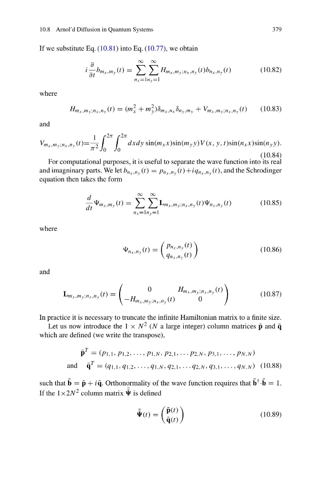
If we substitute Eq. (10.81) into Eq. (10.77), we obtain
i
∂
∂t
b m x ,m y (t) =
∞
n x =1
∞
n y =1
H m x ,m y ;n x ,n y (t)b n x ,n y (t)
(10.82)
where
H m x ,m y ;n x ,n y (t) = (m
2
x + m
2
y )δ m x ,n x δ n y ,m y + V m x ,m y ;n x ,n y (t)
(10.83)
and
V m x ,m y ;n x ,n y (t)=
1
π 2
2π
0
2π
0
dxdy sin(m x x)sin(m y y)V (x, y, t)sin(n x x)sin(n y y).
(10.84)
For computational purposes, it is useful to separate the wave function into its real
and imagninary parts. We let b n x ,n y (t) = p n x ,n y (t)+iq n x ,n y (t), and the Schrodinger
equation then takes the form
d
dt
m x ,m y (t) =
∞
n x =1
∞
n y =1
L m x ,m y ;n x ,n y (t)) n x ,n y (t)
(10.85)
where
n x ,n y (t) =
p n x ,n y (t)
q n x ,n y (t)
(10.86)
and
L m x ,m y ;n x ,n y (t) =
0
H m x ,m y ;n x ,n y (t)
−H m x ,m y ;n x ,n y (t)
0
(10.87)
In practice it is necessary to truncate the infinite Hamiltonian matrix to a finite size.
Let us now introduce the 1 × N 2 (N a large integer) column matrices ¯
p and ¯
q
which are defined (we write the transpose),
¯
p
T
= (p 1,1 , p 1,2 , . . . , p 1,N , p 2,1 , . . . p 2,N , p 3,1 , . . . , p N,N )
and ¯
q
T
= (q 1,1 , q 1,2 , . . . , q 1,N , q 2,1 , . . . q 2,N , q 3,1 , . . . , q N,N ) (10.88)
such that ¯
b = ¯
p + i ¯
q. Orthonormality of the wave function requires that ¯
b † · ¯
b = 1.
If the 1×2N 2 column matrix ¯ ¯
is defined
¯ ¯
(t) =
¯
p(t)
¯
q(t)
(10.89)
379
If we substitute Eq. (10.81) into Eq. (10.77), we obtain
i
∂
∂t
b m x ,m y (t) =
∞
n x =1
∞
n y =1
H m x ,m y ;n x ,n y (t)b n x ,n y (t)
(10.82)
where
H m x ,m y ;n x ,n y (t) = (m
2
x + m
2
y )δ m x ,n x δ n y ,m y + V m x ,m y ;n x ,n y (t)
(10.83)
and
V m x ,m y ;n x ,n y (t)=
1
π 2
2π
0
2π
0
dxdy sin(m x x)sin(m y y)V (x, y, t)sin(n x x)sin(n y y).
(10.84)
For computational purposes, it is useful to separate the wave function into its real
and imagninary parts. We let b n x ,n y (t) = p n x ,n y (t)+iq n x ,n y (t), and the Schrodinger
equation then takes the form
d
dt
m x ,m y (t) =
∞
n x =1
∞
n y =1
L m x ,m y ;n x ,n y (t)) n x ,n y (t)
(10.85)
where
n x ,n y (t) =
p n x ,n y (t)
q n x ,n y (t)
(10.86)
and
L m x ,m y ;n x ,n y (t) =
0
H m x ,m y ;n x ,n y (t)
−H m x ,m y ;n x ,n y (t)
0
(10.87)
In practice it is necessary to truncate the infinite Hamiltonian matrix to a finite size.
Let us now introduce the 1 × N 2 (N a large integer) column matrices ¯
p and ¯
q
which are defined (we write the transpose),
¯
p
T
= (p 1,1 , p 1,2 , . . . , p 1,N , p 2,1 , . . . p 2,N , p 3,1 , . . . , p N,N )
and ¯
q
T
= (q 1,1 , q 1,2 , . . . , q 1,N , q 2,1 , . . . q 2,N , q 3,1 , . . . , q N,N ) (10.88)
such that ¯
b = ¯
p + i ¯
q. Orthonormality of the wave function requires that ¯
b † · ¯
b = 1.
If the 1×2N 2 column matrix ¯ ¯
is defined
¯ ¯
(t) =
¯
p(t)
¯
q(t)
(10.89)