

10.7 Microwave-Driven Hydrogen
375
i
∂ψ n (τ )
∂τ
=
−1
2n 2 ψ n (τ ) −
1
2
λ{z n,n+m e
iω 0 τ ψ n+m (τ )
+z n,n−m e
−iω 0 τ ψ n−m (τ )}.
(10.70)
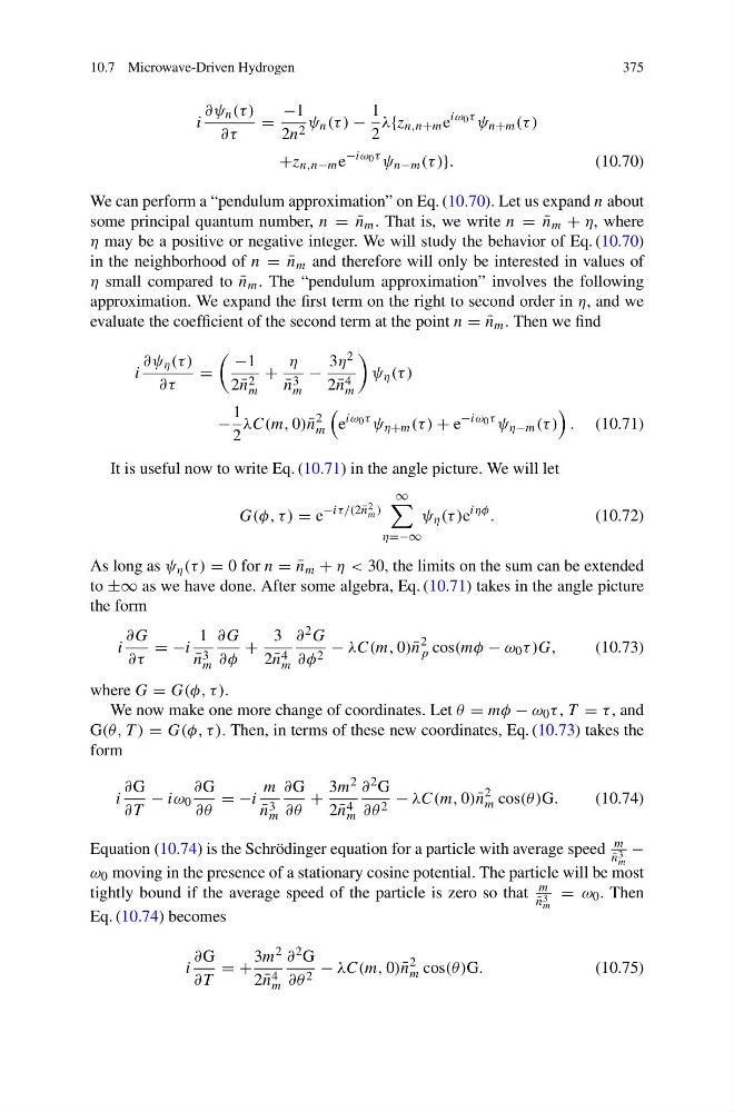
We can perform a “pendulum approximation” on Eq. (10.70). Let us expand n about
some principal quantum number, n = ¯
n m . That is, we write n = ¯
n m + η, where
η may be a positive or negative integer. We will study the behavior of Eq. (10.70)
in the neighborhood of n = ¯
n m and therefore will only be interested in values of
η small compared to ¯
n m . The “pendulum approximation” involves the following
approximation. We expand the first term on the right to second order in η, and we
evaluate the coefficient of the second term at the point n = ¯
n m . Then we find
i
∂ψ η (τ )
∂τ
=
−1
2 ¯
n 2
m
+
η
¯
n 3
m
−
3η 2
2 ¯
n 4
m
ψ η (τ )
−
1
2
λC(m, 0) ¯
n
2
m
e
iω 0 τ ψ η+m (τ ) + e
−iω 0 τ ψ η−m (τ )
. (10.71)
It is useful now to write Eq. (10.71) in the angle picture. We will let
G(φ, τ ) = e
−iτ/(2 ¯
n 2
m )
∞
η=−∞
ψ η (τ )e
iηφ .
(10.72)
As long as ψ η (τ ) = 0 for n = ¯
n m + η < 30, the limits on the sum can be extended
to ±∞ as we have done. After some algebra, Eq. (10.71) takes in the angle picture
the form
i
∂G
∂τ
= −i
1
¯
n 3
m
∂G
∂φ
+
3
2 ¯
n 4
m
∂ 2 G
∂φ 2 − λC(m, 0) ¯
n
2
p cos(mφ − ω 0 τ )G,
(10.73)
where G = G(φ, τ ).
We now make one more change of coordinates. Let θ = mφ − ω 0 τ , T = τ , and
G(θ, T ) = G(φ, τ ). Then, in terms of these new coordinates, Eq. (10.73) takes the
form
i
∂G
∂T
− iω 0
∂G
∂θ
= −i
m
¯
n 3
m
∂G
∂θ
+
3m 2
2 ¯
n 4
m
∂ 2 G
∂θ 2 − λC(m, 0) ¯
n
2
m cos(θ )G.
(10.74)
Equation (10.74) is the Schrödinger equation for a particle with average speed
m
¯
n 3
m
−
ω 0 moving in the presence of a stationary cosine potential. The particle will be most
tightly bound if the average speed of the particle is zero so that
m
¯
n 3
m
= ω 0 . Then
Eq. (10.74) becomes
i
∂G
∂T
= +
3m 2
2 ¯
n 4
m
∂ 2 G
∂θ 2 − λC(m, 0) ¯
n
2
m cos(θ )G.
(10.75)
375
i
∂ψ n (τ )
∂τ
=
−1
2n 2 ψ n (τ ) −
1
2
λ{z n,n+m e
iω 0 τ ψ n+m (τ )
+z n,n−m e
−iω 0 τ ψ n−m (τ )}.
(10.70)
We can perform a “pendulum approximation” on Eq. (10.70). Let us expand n about
some principal quantum number, n = ¯
n m . That is, we write n = ¯
n m + η, where
η may be a positive or negative integer. We will study the behavior of Eq. (10.70)
in the neighborhood of n = ¯
n m and therefore will only be interested in values of
η small compared to ¯
n m . The “pendulum approximation” involves the following
approximation. We expand the first term on the right to second order in η, and we
evaluate the coefficient of the second term at the point n = ¯
n m . Then we find
i
∂ψ η (τ )
∂τ
=
−1
2 ¯
n 2
m
+
η
¯
n 3
m
−
3η 2
2 ¯
n 4
m
ψ η (τ )
−
1
2
λC(m, 0) ¯
n
2
m
e
iω 0 τ ψ η+m (τ ) + e
−iω 0 τ ψ η−m (τ )
. (10.71)
It is useful now to write Eq. (10.71) in the angle picture. We will let
G(φ, τ ) = e
−iτ/(2 ¯
n 2
m )
∞
η=−∞
ψ η (τ )e
iηφ .
(10.72)
As long as ψ η (τ ) = 0 for n = ¯
n m + η < 30, the limits on the sum can be extended
to ±∞ as we have done. After some algebra, Eq. (10.71) takes in the angle picture
the form
i
∂G
∂τ
= −i
1
¯
n 3
m
∂G
∂φ
+
3
2 ¯
n 4
m
∂ 2 G
∂φ 2 − λC(m, 0) ¯
n
2
p cos(mφ − ω 0 τ )G,
(10.73)
where G = G(φ, τ ).
We now make one more change of coordinates. Let θ = mφ − ω 0 τ , T = τ , and
G(θ, T ) = G(φ, τ ). Then, in terms of these new coordinates, Eq. (10.73) takes the
form
i
∂G
∂T
− iω 0
∂G
∂θ
= −i
m
¯
n 3
m
∂G
∂θ
+
3m 2
2 ¯
n 4
m
∂ 2 G
∂θ 2 − λC(m, 0) ¯
n
2
m cos(θ )G.
(10.74)
Equation (10.74) is the Schrödinger equation for a particle with average speed
m
¯
n 3
m
−
ω 0 moving in the presence of a stationary cosine potential. The particle will be most
tightly bound if the average speed of the particle is zero so that
m
¯
n 3
m
= ω 0 . Then
Eq. (10.74) becomes
i
∂G
∂T
= +
3m 2
2 ¯
n 4
m
∂ 2 G
∂θ 2 − λC(m, 0) ¯
n
2
m cos(θ )G.
(10.75)