

376
10 Time-Periodic Quantum Systems
With the choice
m
¯
n 3
m
= ω 0 or equivalently ¯
n m =
m
ω 0
1/3
, the principal quantum
number n = ¯
n m lies right at the center of the mth primary resonance zone. This is
the resonance condition. Equation (10.75) is the Schrödinger equation for a particle
of “mass” m =
¯
n 4
m
3m 2 moving in the presence of the cosine potential with “amplitude”
V = 2
λC(m, 0) ¯
n 2
m . The half-width of the resonance zone for that case is 2
√
mV .
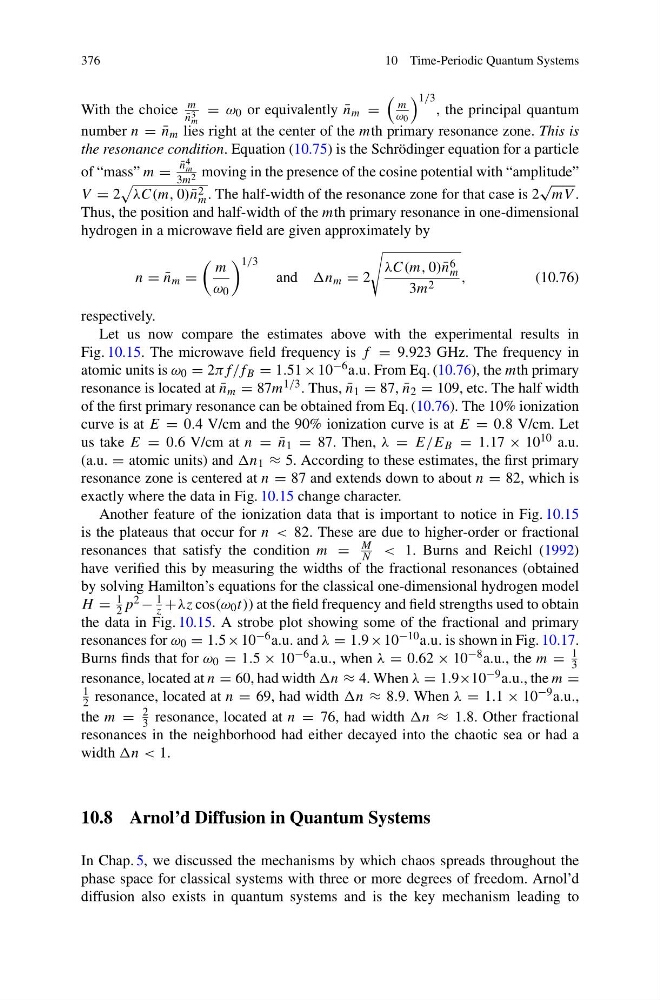
Thus, the position and half-width of the mth primary resonance in one-dimensional
hydrogen in a microwave field are given approximately by
n = ¯
n m =
m
ω 0
1/3
and n m = 2
λC(m, 0) ¯
n 6
m
3m 2
,
(10.76)
respectively.
Let us now compare the estimates above with the experimental results in
Fig. 10.15. The microwave field frequency is f = 9.923 GHz. The frequency in
atomic units is ω 0 = 2πf/f B = 1.51 × 10 −6 a.u. From Eq. (10.76), the mth primary
resonance is located at ¯
n m = 87m 1/3 . Thus, ¯
n 1 = 87, ¯
n 2 = 109, etc. The half width
of the first primary resonance can be obtained from Eq. (10.76). The 10% ionization
curve is at E = 0.4 V/cm and the 90% ionization curve is at E = 0.8 V/cm. Let
us take E = 0.6 V/cm at n = ¯
n 1 = 87. Then, λ = E/E B = 1.17 × 10 10 a.u.
(a.u. = atomic units) and n 1 ≈ 5. According to these estimates, the first primary
resonance zone is centered at n = 87 and extends down to about n = 82, which is
exactly where the data in Fig. 10.15 change character.
Another feature of the ionization data that is important to notice in Fig. 10.15
is the plateaus that occur for n < 82. These are due to higher-order or fractional
resonances that satisfy the condition m =
M
N < 1. Burns and Reichl (1992)
have verified this by measuring the widths of the fractional resonances (obtained
by solving Hamilton’s equations for the classical one-dimensional hydrogen model
H =
1
2 p 2 −
1
z +λz cos(ω 0 t)) at the field frequency and field strengths used to obtain
the data in Fig. 10.15. A strobe plot showing some of the fractional and primary
resonances for ω 0 = 1.5 × 10 −6 a.u. and λ = 1.9 × 10 −10 a.u. is shown in Fig. 10.17.
Burns finds that for ω 0 = 1.5 × 10 −6 a.u., when λ = 0.62 × 10 −8 a.u., the m =
1
3
resonance, located at n = 60, had width n ≈ 4. When λ = 1.9×10 −9 a.u., the m =
1
2 resonance, located at n = 69, had width n ≈ 8.9. When λ = 1.1 × 10 −9 a.u.,
the m =
2
3 resonance, located at n = 76, had width n ≈ 1.8. Other fractional
resonances in the neighborhood had either decayed into the chaotic sea or had a
width n < 1.
10.8 Arnol’d Diffusion in Quantum Systems
In Chap. 5, we discussed the mechanisms by which chaos spreads throughout the
phase space for classical systems with three or more degrees of freedom. Arnol’d
diffusion also exists in quantum systems and is the key mechanism leading to
10 Time-Periodic Quantum Systems
With the choice
m
¯
n 3
m
= ω 0 or equivalently ¯
n m =
m
ω 0
1/3
, the principal quantum
number n = ¯
n m lies right at the center of the mth primary resonance zone. This is
the resonance condition. Equation (10.75) is the Schrödinger equation for a particle
of “mass” m =
¯
n 4
m
3m 2 moving in the presence of the cosine potential with “amplitude”
V = 2
λC(m, 0) ¯
n 2
m . The half-width of the resonance zone for that case is 2
√
mV .
Thus, the position and half-width of the mth primary resonance in one-dimensional
hydrogen in a microwave field are given approximately by
n = ¯
n m =
m
ω 0
1/3
and n m = 2
λC(m, 0) ¯
n 6
m
3m 2
,
(10.76)
respectively.
Let us now compare the estimates above with the experimental results in
Fig. 10.15. The microwave field frequency is f = 9.923 GHz. The frequency in
atomic units is ω 0 = 2πf/f B = 1.51 × 10 −6 a.u. From Eq. (10.76), the mth primary
resonance is located at ¯
n m = 87m 1/3 . Thus, ¯
n 1 = 87, ¯
n 2 = 109, etc. The half width
of the first primary resonance can be obtained from Eq. (10.76). The 10% ionization
curve is at E = 0.4 V/cm and the 90% ionization curve is at E = 0.8 V/cm. Let
us take E = 0.6 V/cm at n = ¯
n 1 = 87. Then, λ = E/E B = 1.17 × 10 10 a.u.
(a.u. = atomic units) and n 1 ≈ 5. According to these estimates, the first primary
resonance zone is centered at n = 87 and extends down to about n = 82, which is
exactly where the data in Fig. 10.15 change character.
Another feature of the ionization data that is important to notice in Fig. 10.15
is the plateaus that occur for n < 82. These are due to higher-order or fractional
resonances that satisfy the condition m =
M
N < 1. Burns and Reichl (1992)
have verified this by measuring the widths of the fractional resonances (obtained
by solving Hamilton’s equations for the classical one-dimensional hydrogen model
H =
1
2 p 2 −
1
z +λz cos(ω 0 t)) at the field frequency and field strengths used to obtain
the data in Fig. 10.15. A strobe plot showing some of the fractional and primary
resonances for ω 0 = 1.5 × 10 −6 a.u. and λ = 1.9 × 10 −10 a.u. is shown in Fig. 10.17.
Burns finds that for ω 0 = 1.5 × 10 −6 a.u., when λ = 0.62 × 10 −8 a.u., the m =
1
3
resonance, located at n = 60, had width n ≈ 4. When λ = 1.9×10 −9 a.u., the m =
1
2 resonance, located at n = 69, had width n ≈ 8.9. When λ = 1.1 × 10 −9 a.u.,
the m =
2
3 resonance, located at n = 76, had width n ≈ 1.8. Other fractional
resonances in the neighborhood had either decayed into the chaotic sea or had a
width n < 1.
10.8 Arnol’d Diffusion in Quantum Systems
In Chap. 5, we discussed the mechanisms by which chaos spreads throughout the
phase space for classical systems with three or more degrees of freedom. Arnol’d
diffusion also exists in quantum systems and is the key mechanism leading to