

2.4 Poincaré Surface of Section
21
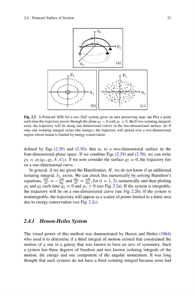
Fig. 2.2 A Poincaré SOS for a two DoF system gives an area preserving map. (a) Plot a point
each time the trajectory passes through the plane q 1 = 0 with p 1 ≥ 0. (b) If two isolating integrals
exist, the trajectory will lie along one-dimensional curves in the two-dimensional surface. (c) If
only one isolating integral exists (the energy), the trajectory will spread over a two-dimensional
region whose extent is limited by energy conservation
defined by Eqs. (2.29) and (2.30); that is, to a two-dimensional surface in the
four-dimensional phase space. If we combine Eqs. (2.29) and (2.30), we can write
p 1 = p 1 (q 1 , q 2 , E, C 2 ). If we now consider the surface q 2 = 0, the trajectory lies
on a one-dimensional curve.
In general, if we are given the Hamiltonian, H , we do not know if an additional
isolating integral, I 2 , exists. We can check this numerically by solving Hamilton’s
equations,
dp i
dt = −
∂H
∂q i
and
dq i
dt =
∂H
∂p i
, for (i = 1, 2), numerically and then plotting
p 2 and q 2 each time q 1 = 0 and p 1 ≥ 0 (see Fig. 2.2a). If the system is integrable,
the trajectory will lie on a one-dimensional curve (see Fig. 2.2b). If the system is
nonintegrable, the trajectory will appear as a scatter of points limited to a finite area
due to energy conservation (see Fig. 2.2c).
2.4.1 Henon-Heiles System
The visual power of this method was demonstrated by Henon and Heiles (1964)
who used it to determine if a third integral of motion existed that constrained the
motion of a star in a galaxy that was known to have an axis of symmetry. Such
a system has three degrees of freedom and two known isolating integrals of the
motion, the energy and one component of the angular momentum. It was long
thought that such systems do not have a third isolating integral because none had
21
Fig. 2.2 A Poincaré SOS for a two DoF system gives an area preserving map. (a) Plot a point
each time the trajectory passes through the plane q 1 = 0 with p 1 ≥ 0. (b) If two isolating integrals
exist, the trajectory will lie along one-dimensional curves in the two-dimensional surface. (c) If
only one isolating integral exists (the energy), the trajectory will spread over a two-dimensional
region whose extent is limited by energy conservation
defined by Eqs. (2.29) and (2.30); that is, to a two-dimensional surface in the
four-dimensional phase space. If we combine Eqs. (2.29) and (2.30), we can write
p 1 = p 1 (q 1 , q 2 , E, C 2 ). If we now consider the surface q 2 = 0, the trajectory lies
on a one-dimensional curve.
In general, if we are given the Hamiltonian, H , we do not know if an additional
isolating integral, I 2 , exists. We can check this numerically by solving Hamilton’s
equations,
dp i
dt = −
∂H
∂q i
and
dq i
dt =
∂H
∂p i
, for (i = 1, 2), numerically and then plotting
p 2 and q 2 each time q 1 = 0 and p 1 ≥ 0 (see Fig. 2.2a). If the system is integrable,
the trajectory will lie on a one-dimensional curve (see Fig. 2.2b). If the system is
nonintegrable, the trajectory will appear as a scatter of points limited to a finite area
due to energy conservation (see Fig. 2.2c).
2.4.1 Henon-Heiles System
The visual power of this method was demonstrated by Henon and Heiles (1964)
who used it to determine if a third integral of motion existed that constrained the
motion of a star in a galaxy that was known to have an axis of symmetry. Such
a system has three degrees of freedom and two known isolating integrals of the
motion, the energy and one component of the angular momentum. It was long
thought that such systems do not have a third isolating integral because none had