

308
9 Semiclassical Theory: Path Integrals
9.5.1 General Expression
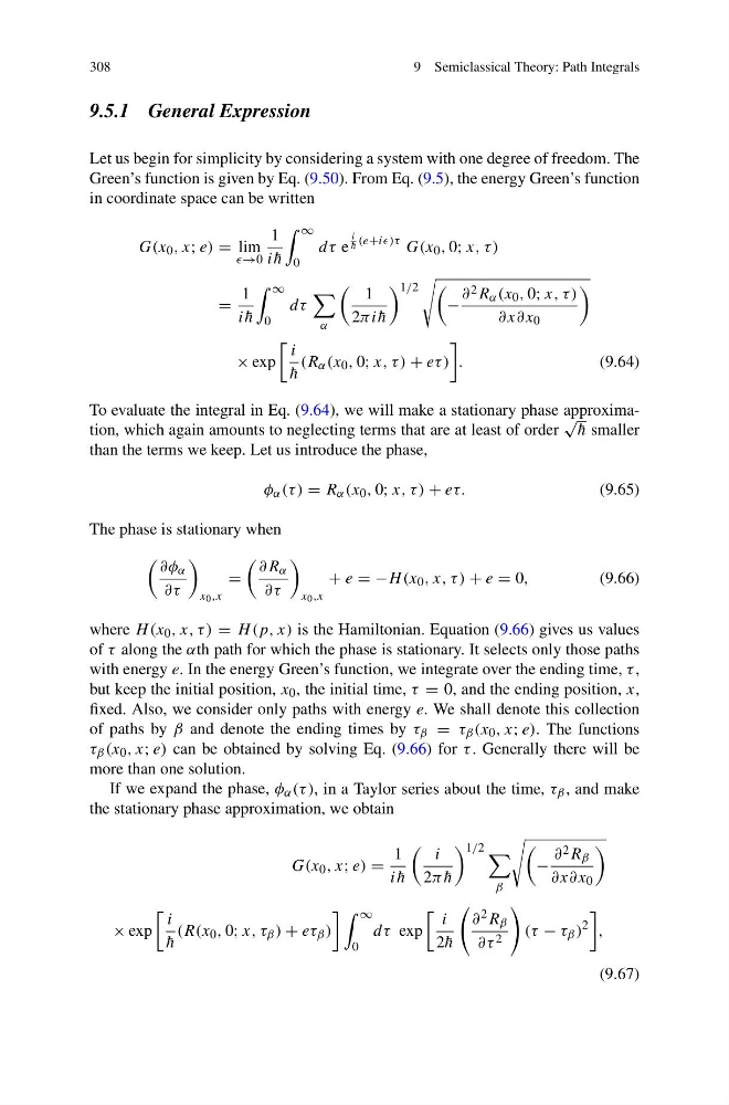
Let us begin for simplicity by considering a system with one degree of freedom. The
Green’s function is given by Eq. (9.50). From Eq. (9.5), the energy Green’s function
in coordinate space can be written
G(x 0 , x; e) = lim
→0
1
i ¯
h
∞
0
dτ e
i
¯
h (e+ii)τ G(x 0 , 0; x, τ )
=
1
i ¯
h
∞
0
dτ
α
1
2πi ¯
h
1/2
−
∂ 2 R α (x 0 , 0; x, τ )
∂x∂x 0
× exp
i
¯
h
(R α (x 0 , 0; x, τ ) + eτ )
.
(9.64)
To evaluate the integral in Eq. (9.64), we will make a stationary phase approximation, which again amounts to neglecting terms that are at least of order
√ ¯
h smaller
than the terms we keep. Let us introduce the phase,
φ α (τ ) = R α (x 0 , 0; x, τ ) + eτ.
(9.65)
The phase is stationary when
∂φ α
∂τ
x 0 ,x
=
∂R α
∂τ
x 0 ,x
+ e = −H (x 0 , x, τ ) + e = 0,
(9.66)
where H (x 0 , x, τ ) = H (p, x) is the Hamiltonian. Equation (9.66) gives us values
of τ along the αth path for which the phase is stationary. It selects only those paths
with energy e. In the energy Green’s function, we integrate over the ending time, τ ,
but keep the initial position, x 0 , the initial time, τ = 0, and the ending position, x,
fixed. Also, we consider only paths with energy e. We shall denote this collection
of paths by β and denote the ending times by τ β = τ β (x 0 , x; e). The functions
τ β (x 0 , x; e) can be obtained by solving Eq. (9.66) for τ . Generally there will be
more than one solution.
If we expand the phase, φ α (τ ), in a Taylor series about the time, τ β , and make
the stationary phase approximation, we obtain
G(x 0 , x; e) =
1
i ¯
h
i
2π ¯
h
1/2
β
−
∂ 2 R β
∂x∂x 0
× exp
i
¯
h
(R(x 0 , 0; x, τ β ) + eτ β )
∞
0
dτ exp
i
2 ¯
h
∂ 2 R β
∂τ 2
(τ − τ β )
2
,
(9.67)
9 Semiclassical Theory: Path Integrals
9.5.1 General Expression
Let us begin for simplicity by considering a system with one degree of freedom. The
Green’s function is given by Eq. (9.50). From Eq. (9.5), the energy Green’s function
in coordinate space can be written
G(x 0 , x; e) = lim
→0
1
i ¯
h
∞
0
dτ e
i
¯
h (e+ii)τ G(x 0 , 0; x, τ )
=
1
i ¯
h
∞
0
dτ
α
1
2πi ¯
h
1/2
−
∂ 2 R α (x 0 , 0; x, τ )
∂x∂x 0
× exp
i
¯
h
(R α (x 0 , 0; x, τ ) + eτ )
.
(9.64)
To evaluate the integral in Eq. (9.64), we will make a stationary phase approximation, which again amounts to neglecting terms that are at least of order
√ ¯
h smaller
than the terms we keep. Let us introduce the phase,
φ α (τ ) = R α (x 0 , 0; x, τ ) + eτ.
(9.65)
The phase is stationary when
∂φ α
∂τ
x 0 ,x
=
∂R α
∂τ
x 0 ,x
+ e = −H (x 0 , x, τ ) + e = 0,
(9.66)
where H (x 0 , x, τ ) = H (p, x) is the Hamiltonian. Equation (9.66) gives us values
of τ along the αth path for which the phase is stationary. It selects only those paths
with energy e. In the energy Green’s function, we integrate over the ending time, τ ,
but keep the initial position, x 0 , the initial time, τ = 0, and the ending position, x,
fixed. Also, we consider only paths with energy e. We shall denote this collection
of paths by β and denote the ending times by τ β = τ β (x 0 , x; e). The functions
τ β (x 0 , x; e) can be obtained by solving Eq. (9.66) for τ . Generally there will be
more than one solution.
If we expand the phase, φ α (τ ), in a Taylor series about the time, τ β , and make
the stationary phase approximation, we obtain
G(x 0 , x; e) =
1
i ¯
h
i
2π ¯
h
1/2
β
−
∂ 2 R β
∂x∂x 0
× exp
i
¯
h
(R(x 0 , 0; x, τ β ) + eτ β )
∞
0
dτ exp
i
2 ¯
h
∂ 2 R β
∂τ 2
(τ − τ β )
2
,
(9.67)