

9.5 Energy Green’s Function
309
where R β = R(x 0 , 0; x, τ β ). From Eq. (9.27), we find
G(x 0 , x; e) = ¯
G(x 0 , x; e) + G osc (x 0 , x; e),
where ¯
G(x 0 , x; e) gives an average contribution from very short orbits for which
the stationary phase approximation does not apply and
G osc (x 0 , x; e) =
1
i ¯
h
β
−
∂ 2 R β
∂x∂x 0
/
∂ 2 R β
∂τ 2
× exp
i
¯
h
(R(x 0 , 0; x, τ β ) + eτ β )
(9.68)
gives the stationary phase approximation to oscillatory contributions from longer
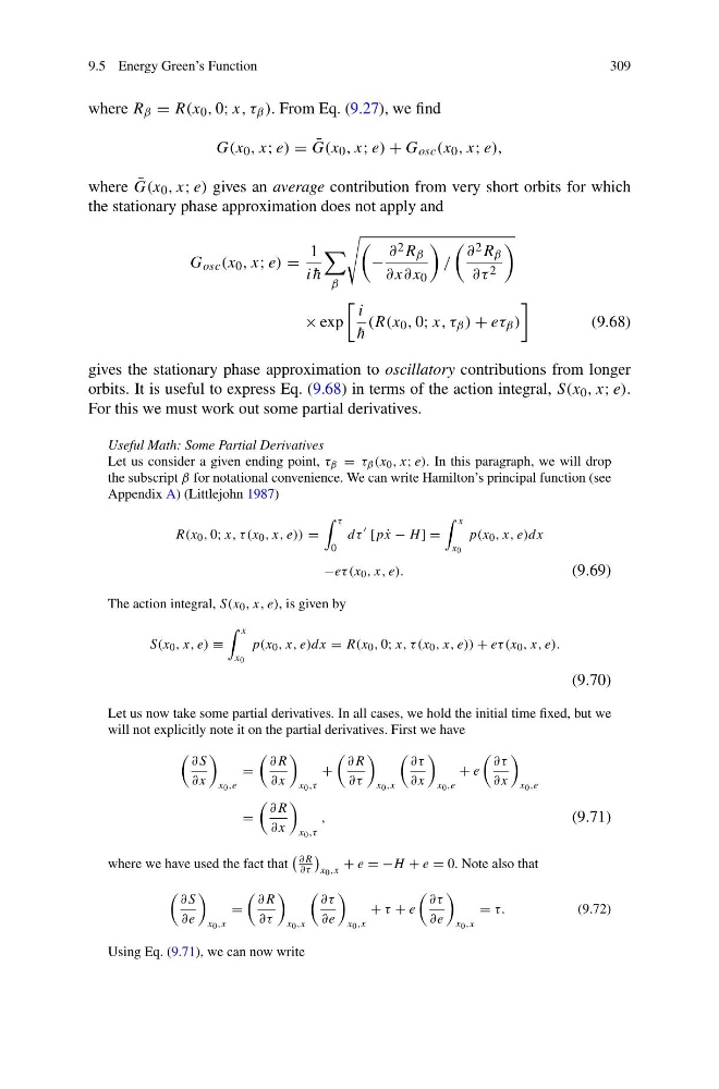
orbits. It is useful to express Eq. (9.68) in terms of the action integral, S(x 0 , x; e).
For this we must work out some partial derivatives.
Useful Math: Some Partial Derivatives
Let us consider a given ending point, τ β = τ β (x 0 , x; e). In this paragraph, we will drop
the subscript β for notational convenience. We can write Hamilton’s principal function (see
Appendix A) (Littlejohn 1987)
R(x 0 , 0; x, τ (x 0 , x, e)) =
τ
0
dτ
[p ˙
x − H ] =
x
x 0
p(x 0 , x, e)dx
−eτ (x 0 , x, e).
(9.69)
The action integral, S(x 0 , x, e), is given by
S(x 0 , x, e) ≡
x
x 0
p(x 0 , x, e)dx = R(x 0 , 0; x, τ (x 0 , x, e)) + eτ (x 0 , x, e).
(9.70)
Let us now take some partial derivatives. In all cases, we hold the initial time fixed, but we
will not explicitly note it on the partial derivatives. First we have
∂S
∂x
x 0 ,e
=
∂R
∂x
x 0 ,τ
+
∂R
∂τ
x 0 ,x
∂τ
∂x
x 0 ,e
+ e
∂τ
∂x
x 0 ,e
=
∂R
∂x
x 0 ,τ
,
(9.71)
where we have used the fact that
∂R
∂τ
x 0 ,x
+ e = −H + e = 0. Note also that
∂S
∂e
x 0 ,x
=
∂R
∂τ
x 0 ,x
∂τ
∂e
x 0 ,x
+ τ + e
∂τ
∂e
x 0 ,x
= τ.
(9.72)
Using Eq. (9.71), we can now write
309
where R β = R(x 0 , 0; x, τ β ). From Eq. (9.27), we find
G(x 0 , x; e) = ¯
G(x 0 , x; e) + G osc (x 0 , x; e),
where ¯
G(x 0 , x; e) gives an average contribution from very short orbits for which
the stationary phase approximation does not apply and
G osc (x 0 , x; e) =
1
i ¯
h
β
−
∂ 2 R β
∂x∂x 0
/
∂ 2 R β
∂τ 2
× exp
i
¯
h
(R(x 0 , 0; x, τ β ) + eτ β )
(9.68)
gives the stationary phase approximation to oscillatory contributions from longer
orbits. It is useful to express Eq. (9.68) in terms of the action integral, S(x 0 , x; e).
For this we must work out some partial derivatives.
Useful Math: Some Partial Derivatives
Let us consider a given ending point, τ β = τ β (x 0 , x; e). In this paragraph, we will drop
the subscript β for notational convenience. We can write Hamilton’s principal function (see
Appendix A) (Littlejohn 1987)
R(x 0 , 0; x, τ (x 0 , x, e)) =
τ
0
dτ
[p ˙
x − H ] =
x
x 0
p(x 0 , x, e)dx
−eτ (x 0 , x, e).
(9.69)
The action integral, S(x 0 , x, e), is given by
S(x 0 , x, e) ≡
x
x 0
p(x 0 , x, e)dx = R(x 0 , 0; x, τ (x 0 , x, e)) + eτ (x 0 , x, e).
(9.70)
Let us now take some partial derivatives. In all cases, we hold the initial time fixed, but we
will not explicitly note it on the partial derivatives. First we have
∂S
∂x
x 0 ,e
=
∂R
∂x
x 0 ,τ
+
∂R
∂τ
x 0 ,x
∂τ
∂x
x 0 ,e
+ e
∂τ
∂x
x 0 ,e
=
∂R
∂x
x 0 ,τ
,
(9.71)
where we have used the fact that
∂R
∂τ
x 0 ,x
+ e = −H + e = 0. Note also that
∂S
∂e
x 0 ,x
=
∂R
∂τ
x 0 ,x
∂τ
∂e
x 0 ,x
+ τ + e
∂τ
∂e
x 0 ,x
= τ.
(9.72)
Using Eq. (9.71), we can now write