

9.5 Energy Green’s Function
307
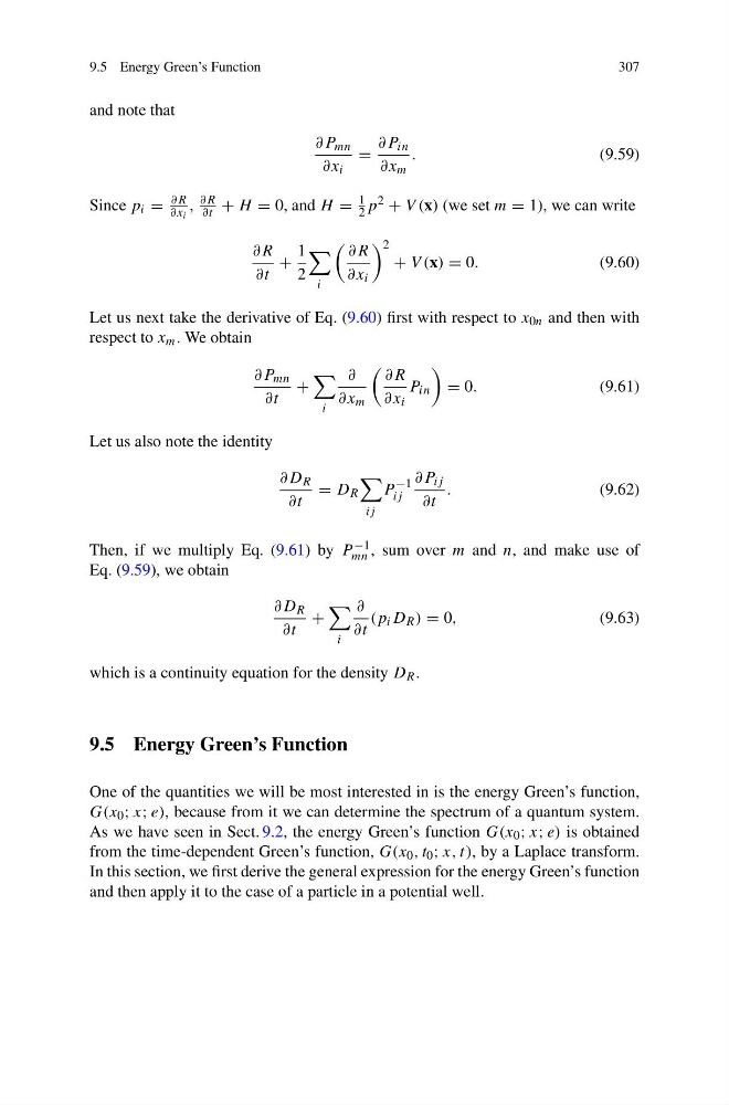
and note that
∂P mn
∂x i
=
∂P in
∂x m
.
(9.59)
Since p i =
∂R
∂x i
,
∂R
∂t + H = 0, and H =
1
2 p 2 + V (x) (we set m = 1), we can write
∂R
∂t
+
1
2
i
∂R
∂x i
2
+ V (x) = 0.
(9.60)
Let us next take the derivative of Eq. (9.60) first with respect to x 0n and then with
respect to x m . We obtain
∂P mn
∂t
+
i
∂
∂x m
∂R
∂x i
P in
= 0.
(9.61)
Let us also note the identity
∂D R
∂t
= D R
ij
P
−1
ij
∂P ij
∂t
.
(9.62)
Then, if we multiply Eq. (9.61) by P −1
mn , sum over m and n, and make use of
Eq. (9.59), we obtain
∂D R
∂t
+
i
∂
∂t
(p i D R ) = 0,
(9.63)
which is a continuity equation for the density D R .
9.5 Energy Green’s Function
One of the quantities we will be most interested in is the energy Green’s function,
G(x 0 ; x; e), because from it we can determine the spectrum of a quantum system.
As we have seen in Sect. 9.2, the energy Green’s function G(x 0 ; x; e) is obtained
from the time-dependent Green’s function, G(x 0 , t 0 ; x, t), by a Laplace transform.
In this section, we first derive the general expression for the energy Green’s function
and then apply it to the case of a particle in a potential well.
307
and note that
∂P mn
∂x i
=
∂P in
∂x m
.
(9.59)
Since p i =
∂R
∂x i
,
∂R
∂t + H = 0, and H =
1
2 p 2 + V (x) (we set m = 1), we can write
∂R
∂t
+
1
2
i
∂R
∂x i
2
+ V (x) = 0.
(9.60)
Let us next take the derivative of Eq. (9.60) first with respect to x 0n and then with
respect to x m . We obtain
∂P mn
∂t
+
i
∂
∂x m
∂R
∂x i
P in
= 0.
(9.61)
Let us also note the identity
∂D R
∂t
= D R
ij
P
−1
ij
∂P ij
∂t
.
(9.62)
Then, if we multiply Eq. (9.61) by P −1
mn , sum over m and n, and make use of
Eq. (9.59), we obtain
∂D R
∂t
+
i
∂
∂t
(p i D R ) = 0,
(9.63)
which is a continuity equation for the density D R .
9.5 Energy Green’s Function
One of the quantities we will be most interested in is the energy Green’s function,
G(x 0 ; x; e), because from it we can determine the spectrum of a quantum system.
As we have seen in Sect. 9.2, the energy Green’s function G(x 0 ; x; e) is obtained
from the time-dependent Green’s function, G(x 0 , t 0 ; x, t), by a Laplace transform.
In this section, we first derive the general expression for the energy Green’s function
and then apply it to the case of a particle in a potential well.