

300
9 Semiclassical Theory: Path Integrals
9.4 Semiclassical Approximation
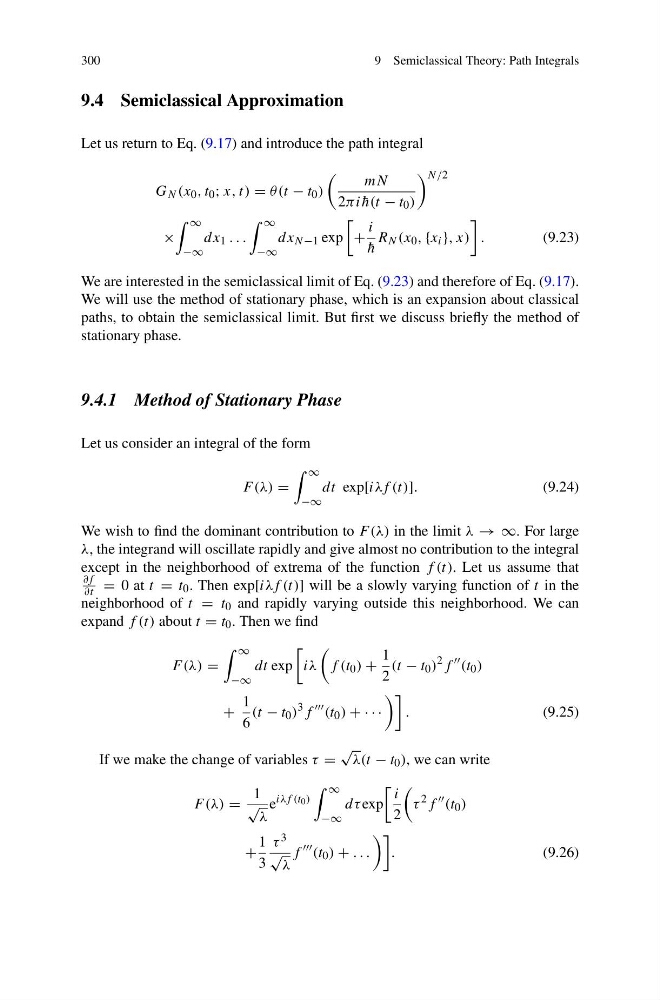
Let us return to Eq. (9.17) and introduce the path integral
G N (x 0 , t 0 ; x, t) = θ(t − t 0 )
mN
2πi ¯
h(t − t 0 )
N/2
×
∞
−∞
dx 1 . . .
∞
−∞
dx N −1 exp
+
i
¯
h
R N (x 0 , {x i }, x)
.
(9.23)
We are interested in the semiclassical limit of Eq. (9.23) and therefore of Eq. (9.17).
We will use the method of stationary phase, which is an expansion about classical
paths, to obtain the semiclassical limit. But first we discuss briefly the method of
stationary phase.
9.4.1 Method of Stationary Phase
Let us consider an integral of the form
F (λ) =
∞
−∞
dt exp[iλf (t)].
(9.24)
We wish to find the dominant contribution to F (λ) in the limit λ → ∞. For large
λ, the integrand will oscillate rapidly and give almost no contribution to the integral
except in the neighborhood of extrema of the function f (t). Let us assume that
∂f
∂t = 0 at t = t 0 . Then exp[iλf (t)] will be a slowly varying function of t in the
neighborhood of t = t 0 and rapidly varying outside this neighborhood. We can
expand f (t) about t = t 0 . Then we find
F (λ) =
∞
−∞
dt exp
iλ
f (t 0 ) +
1
2
(t − t 0 )
2 f
(t 0 )
+
1
6
(t − t 0 )
3 f
(t 0 ) + · · ·
.
(9.25)
If we make the change of variables τ =
√
λ(t − t 0 ), we can write
F (λ) =
1
√
λ
e
iλf (t 0 )
∞
−∞
dτ exp
i
2
τ
2 f
(t 0 )
+
1
3
τ 3
√
λ
f
(t 0 ) + . . .
.
(9.26)
9 Semiclassical Theory: Path Integrals
9.4 Semiclassical Approximation
Let us return to Eq. (9.17) and introduce the path integral
G N (x 0 , t 0 ; x, t) = θ(t − t 0 )
mN
2πi ¯
h(t − t 0 )
N/2
×
∞
−∞
dx 1 . . .
∞
−∞
dx N −1 exp
+
i
¯
h
R N (x 0 , {x i }, x)
.
(9.23)
We are interested in the semiclassical limit of Eq. (9.23) and therefore of Eq. (9.17).
We will use the method of stationary phase, which is an expansion about classical
paths, to obtain the semiclassical limit. But first we discuss briefly the method of
stationary phase.
9.4.1 Method of Stationary Phase
Let us consider an integral of the form
F (λ) =
∞
−∞
dt exp[iλf (t)].
(9.24)
We wish to find the dominant contribution to F (λ) in the limit λ → ∞. For large
λ, the integrand will oscillate rapidly and give almost no contribution to the integral
except in the neighborhood of extrema of the function f (t). Let us assume that
∂f
∂t = 0 at t = t 0 . Then exp[iλf (t)] will be a slowly varying function of t in the
neighborhood of t = t 0 and rapidly varying outside this neighborhood. We can
expand f (t) about t = t 0 . Then we find
F (λ) =
∞
−∞
dt exp
iλ
f (t 0 ) +
1
2
(t − t 0 )
2 f
(t 0 )
+
1
6
(t − t 0 )
3 f
(t 0 ) + · · ·
.
(9.25)
If we make the change of variables τ =
√
λ(t − t 0 ), we can write
F (λ) =
1
√
λ
e
iλf (t 0 )
∞
−∞
dτ exp
i
2
τ
2 f
(t 0 )
+
1
3
τ 3
√
λ
f
(t 0 ) + . . .
.
(9.26)