

9.4 Semiclassical Approximation
301
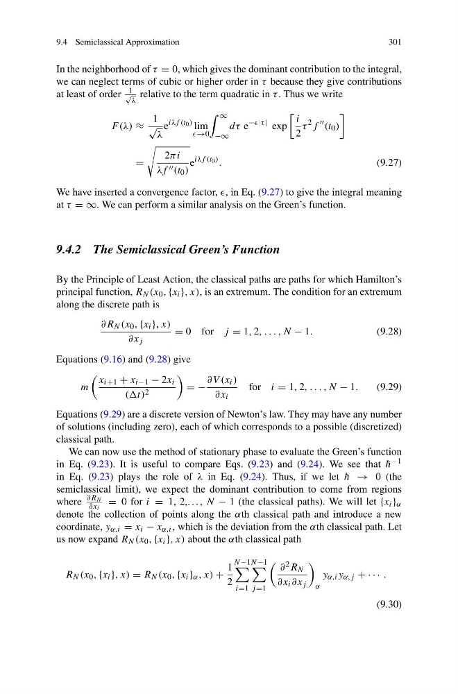
In the neighborhood of τ = 0, which gives the dominant contribution to the integral,
we can neglect terms of cubic or higher order in τ because they give contributions
at least of order
1
√
λ
relative to the term quadratic in τ . Thus we write
F (λ) ≈
1
√
λ
e
iλf (t 0 ) lim
→0
∞
−∞
dτ e
−|τ | exp
i
2
τ
2 f
(t 0 )
=
2πi
λf (t 0 )
e
iλf (t 0 ) .
(9.27)
We have inserted a convergence factor, , in Eq. (9.27) to give the integral meaning
at τ = ∞. We can perform a similar analysis on the Green’s function.
9.4.2 The Semiclassical Green’s Function
By the Principle of Least Action, the classical paths are paths for which Hamilton’s
principal function, R N (x 0 , {x i }, x), is an extremum. The condition for an extremum
along the discrete path is
∂R N (x 0 , {x i }, x)
∂x j
= 0 for j = 1, 2, . . . , N − 1.
(9.28)
Equations (9.16) and (9.28) give
m
x i+1 + x i−1 − 2x i
((t) 2
= −
∂V (x i )
∂x i
for i = 1, 2, . . . , N − 1.
(9.29)
Equations (9.29) are a discrete version of Newton’s law. They may have any number
of solutions (including zero), each of which corresponds to a possible (discretized)
classical path.
We can now use the method of stationary phase to evaluate the Green’s function
in Eq. (9.23). It is useful to compare Eqs. (9.23) and (9.24). We see that ¯
h −1
in Eq. (9.23) plays the role of λ in Eq. (9.24). Thus, if we let ¯
h → 0 (the
semiclassical limit), we expect the dominant contribution to come from regions
where
∂R N
∂x i
= 0 for i = 1, 2,. . . , N − 1 (the classical paths). We will let {x i } α
denote the collection of points along the αth classical path and introduce a new
coordinate, y α,i = x i − x α,i , which is the deviation from the αth classical path. Let
us now expand R N (x 0 , {x i }, x) about the αth classical path
R N (x 0 , {x i }, x) = R N (x 0 , {x i } α , x) +
1
2
N −1
i=1
N −1
j =1
∂ 2 R N
∂x i ∂x j
α
y α,i y α,j + · · · .
(9.30)
301
In the neighborhood of τ = 0, which gives the dominant contribution to the integral,
we can neglect terms of cubic or higher order in τ because they give contributions
at least of order
1
√
λ
relative to the term quadratic in τ . Thus we write
F (λ) ≈
1
√
λ
e
iλf (t 0 ) lim
→0
∞
−∞
dτ e
−|τ | exp
i
2
τ
2 f
(t 0 )
=
2πi
λf (t 0 )
e
iλf (t 0 ) .
(9.27)
We have inserted a convergence factor, , in Eq. (9.27) to give the integral meaning
at τ = ∞. We can perform a similar analysis on the Green’s function.
9.4.2 The Semiclassical Green’s Function
By the Principle of Least Action, the classical paths are paths for which Hamilton’s
principal function, R N (x 0 , {x i }, x), is an extremum. The condition for an extremum
along the discrete path is
∂R N (x 0 , {x i }, x)
∂x j
= 0 for j = 1, 2, . . . , N − 1.
(9.28)
Equations (9.16) and (9.28) give
m
x i+1 + x i−1 − 2x i
((t) 2
= −
∂V (x i )
∂x i
for i = 1, 2, . . . , N − 1.
(9.29)
Equations (9.29) are a discrete version of Newton’s law. They may have any number
of solutions (including zero), each of which corresponds to a possible (discretized)
classical path.
We can now use the method of stationary phase to evaluate the Green’s function
in Eq. (9.23). It is useful to compare Eqs. (9.23) and (9.24). We see that ¯
h −1
in Eq. (9.23) plays the role of λ in Eq. (9.24). Thus, if we let ¯
h → 0 (the
semiclassical limit), we expect the dominant contribution to come from regions
where
∂R N
∂x i
= 0 for i = 1, 2,. . . , N − 1 (the classical paths). We will let {x i } α
denote the collection of points along the αth classical path and introduce a new
coordinate, y α,i = x i − x α,i , which is the deviation from the αth classical path. Let
us now expand R N (x 0 , {x i }, x) about the αth classical path
R N (x 0 , {x i }, x) = R N (x 0 , {x i } α , x) +
1
2
N −1
i=1
N −1
j =1
∂ 2 R N
∂x i ∂x j
α
y α,i y α,j + · · · .
(9.30)