

296
9 Semiclassical Theory: Path Integrals
In Eq. (9.3), θ(t − t 0 ) is the Heaviside function (defined θ(x) = 1 for x > 0 and
θ(x) = 0 for x < 0) and ensures that |D(t) can only affect the wave function at
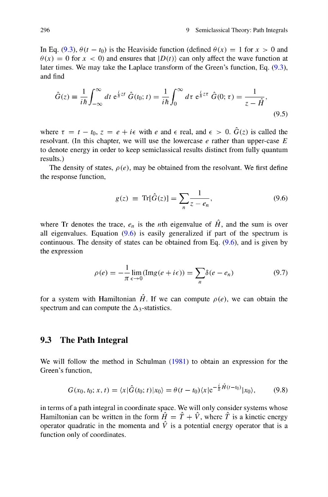
later times. We may take the Laplace transform of the Green’s function, Eq. (9.3),
and find
ˆ
G(z) ≡
1
i ¯
h
∞
−∞
dt e
i
¯
h zt ˆ
G(t 0 ; t) =
1
i ¯
h
∞
0
dτ e
i
¯
h zτ ˆ
G(0; τ ) =
1
z − ˆ
H
,
(9.5)
where τ = t − t 0 , z = e + ii with e and real, and > 0. ˆ
G(z) is called the
resolvant. (In this chapter, we will use the lowercase e rather than upper-case E
to denote energy in order to keep semiclassical results distinct from fully quantum
results.)
The density of states, ρ(e), may be obtained from the resolvant. We first define
the response function,
g(z) ≡ Tr[ ˆ
G(z)] =
n
1
z − e n
,
(9.6)
where Tr denotes the trace, e n is the nth eigenvalue of ˆ
H , and the sum is over
all eigenvalues. Equation (9.6) is easily generalized if part of the spectrum is
continuous. The density of states can be obtained from Eq. (9.6), and is given by
the expression
ρ(e) = −
1
π
lim
→0
(Img(e + ii)) =
n
δ(e − e n )
(9.7)
for a system with Hamiltonian ˆ
H . If we can compute ρ(e), we can obtain the
spectrum and can compute the 3 -statistics.
9.3 The Path Integral
We will follow the method in Schulman (1981) to obtain an expression for the
Green’s function,
G(x 0 , t 0 ; x, t) = =x| ˆ
G(t 0 ; t)|x 0 = θ(t − t 0 )x|e
−
i
¯
h
ˆ
H (t−t 0 ) |x 0 ,
(9.8)
in terms of a path integral in coordinate space. We will only consider systems whose
Hamiltonian can be written in the form ˆ
H = ˆ
T + ˆ
V , where ˆ
T is a kinetic energy
operator quadratic in the momenta and ˆ
V is a potential energy operator that is a
function only of coordinates.
9 Semiclassical Theory: Path Integrals
In Eq. (9.3), θ(t − t 0 ) is the Heaviside function (defined θ(x) = 1 for x > 0 and
θ(x) = 0 for x < 0) and ensures that |D(t) can only affect the wave function at
later times. We may take the Laplace transform of the Green’s function, Eq. (9.3),
and find
ˆ
G(z) ≡
1
i ¯
h
∞
−∞
dt e
i
¯
h zt ˆ
G(t 0 ; t) =
1
i ¯
h
∞
0
dτ e
i
¯
h zτ ˆ
G(0; τ ) =
1
z − ˆ
H
,
(9.5)
where τ = t − t 0 , z = e + ii with e and real, and > 0. ˆ
G(z) is called the
resolvant. (In this chapter, we will use the lowercase e rather than upper-case E
to denote energy in order to keep semiclassical results distinct from fully quantum
results.)
The density of states, ρ(e), may be obtained from the resolvant. We first define
the response function,
g(z) ≡ Tr[ ˆ
G(z)] =
n
1
z − e n
,
(9.6)
where Tr denotes the trace, e n is the nth eigenvalue of ˆ
H , and the sum is over
all eigenvalues. Equation (9.6) is easily generalized if part of the spectrum is
continuous. The density of states can be obtained from Eq. (9.6), and is given by
the expression
ρ(e) = −
1
π
lim
→0
(Img(e + ii)) =
n
δ(e − e n )
(9.7)
for a system with Hamiltonian ˆ
H . If we can compute ρ(e), we can obtain the
spectrum and can compute the 3 -statistics.
9.3 The Path Integral
We will follow the method in Schulman (1981) to obtain an expression for the
Green’s function,
G(x 0 , t 0 ; x, t) = =x| ˆ
G(t 0 ; t)|x 0 = θ(t − t 0 )x|e
−
i
¯
h
ˆ
H (t−t 0 ) |x 0 ,
(9.8)
in terms of a path integral in coordinate space. We will only consider systems whose
Hamiltonian can be written in the form ˆ
H = ˆ
T + ˆ
V , where ˆ
T is a kinetic energy
operator quadratic in the momenta and ˆ
V is a potential energy operator that is a
function only of coordinates.