

282
8 Manifestations of Chaos in Quantum Scattering Processes
¯
S
o
M = ˜
C N π
N(N+1)/2
∞
−∞
. . .
∞
−∞
dd H N
¯
S o
M
det[π 2 ¯
1 N + ( ¯
H N ) 2 ] (N +1)/2
.
(8.145)
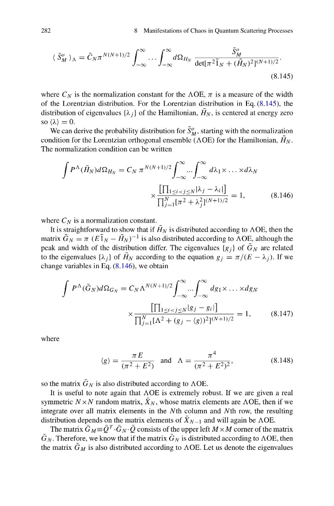
where C N is the normalization constant for the OE, π is a measure of the width
of the Lorentzian distribution. For the Lorentzian distribution in Eq. (8.145), the
distribution of eigenvalues {λ j } of the Hamiltonian, ¯
H N , is centered at energy zero
so λ = 0.
We can derive the probability distribution for ¯
S o
M , starting with the normalization
condition for the Lorentzian orthogonal ensemble (OE) for the Hamiltonian, ¯
H N .
The normalization condition can be written
P
( ¯
H N )dd H N = C N π
N(N+1)/2
∞
−∞
...
∞
−∞
dλ 1 × . . . ×dλ N
×
1≤i
j =1 [π 2 + λ 2
j ] (N +1)/2
= 1,
(8.146)
where C N is a normalization constant.
It is straightforward to show that if ¯
H N is distributed according to OE, then the
matrix ¯
G N = π (E ¯
1 N − ¯
H N ) −1 is also distributed according to OE, although the
peak and width of the distribution differ. The eigenvalues {g j } of ¯
G N are related
to the eigenvalues {λ j } of ¯
H N according to the equation g j = π/(E − λ j ). If we
change variables in Eq. (8.146), we obtain
P
( ¯
G N )dd G N = C N
N(N+1)/2
∞
−∞
...
∞
−∞
dg 1 × . . . ×dg N
×
1≤i
j =1 [ 2 + (g j − −g) 2 ] (N +1)/2
= 1,
(8.147)
where
g =
πE
(π 2 + E 2 )
and =
π 4
(π 2 + E 2 ) 2 ,
(8.148)
so the matrix ¯
G N is also distributed according to OE.
It is useful to note again that OE is extremely robust. If we are given a real
symmetric N ×N random matrix, ¯
X N , whose matrix elements are OE, then if we
integrate over all matrix elements in the Nth column and N th row, the resulting
distribution depends on the matrix elements of ¯
X N −1 and will again be OE.
The matrix ¯
G M ≡ ¯
Q T · ¯
G N · ¯
Q consists of the upper left M×M corner of the matrix
¯
G N . Therefore, we know that if the matrix ¯
G N is distributed according to OE, then
the matrix ¯
G M is also distributed according to OE. Let us denote the eigenvalues
8 Manifestations of Chaos in Quantum Scattering Processes
¯
S
o
M = ˜
C N π
N(N+1)/2
∞
−∞
. . .
∞
−∞
dd H N
¯
S o
M
det[π 2 ¯
1 N + ( ¯
H N ) 2 ] (N +1)/2
.
(8.145)
where C N is the normalization constant for the OE, π is a measure of the width
of the Lorentzian distribution. For the Lorentzian distribution in Eq. (8.145), the
distribution of eigenvalues {λ j } of the Hamiltonian, ¯
H N , is centered at energy zero
so λ = 0.
We can derive the probability distribution for ¯
S o
M , starting with the normalization
condition for the Lorentzian orthogonal ensemble (OE) for the Hamiltonian, ¯
H N .
The normalization condition can be written
P
( ¯
H N )dd H N = C N π
N(N+1)/2
∞
−∞
...
∞
−∞
dλ 1 × . . . ×dλ N
×
1≤i
j =1 [π 2 + λ 2
j ] (N +1)/2
= 1,
(8.146)
where C N is a normalization constant.
It is straightforward to show that if ¯
H N is distributed according to OE, then the
matrix ¯
G N = π (E ¯
1 N − ¯
H N ) −1 is also distributed according to OE, although the
peak and width of the distribution differ. The eigenvalues {g j } of ¯
G N are related
to the eigenvalues {λ j } of ¯
H N according to the equation g j = π/(E − λ j ). If we
change variables in Eq. (8.146), we obtain
P
( ¯
G N )dd G N = C N
N(N+1)/2
∞
−∞
...
∞
−∞
dg 1 × . . . ×dg N
×
1≤i
j =1 [ 2 + (g j − −g) 2 ] (N +1)/2
= 1,
(8.147)
where
g =
πE
(π 2 + E 2 )
and =
π 4
(π 2 + E 2 ) 2 ,
(8.148)
so the matrix ¯
G N is also distributed according to OE.
It is useful to note again that OE is extremely robust. If we are given a real
symmetric N ×N random matrix, ¯
X N , whose matrix elements are OE, then if we
integrate over all matrix elements in the Nth column and N th row, the resulting
distribution depends on the matrix elements of ¯
X N −1 and will again be OE.
The matrix ¯
G M ≡ ¯
Q T · ¯
G N · ¯
Q consists of the upper left M×M corner of the matrix
¯
G N . Therefore, we know that if the matrix ¯
G N is distributed according to OE, then
the matrix ¯
G M is also distributed according to OE. Let us denote the eigenvalues