

8.6 COE and GOE
281
8.6.4 When Does a GOE Hamiltonian Yield a COE S-Matrix?
In 1995, Brouwer gave an indirect proof (Brouwer 1995) that, in the limit N→∞,
an N ×N GOE Hamiltonian, ¯
H N , gives an M×M COE S-matrix (keeping M <
N ). Brouwer’s proof uses the Lorentzian orthogonal ensemble (OE) in the limit
N →∞ (keeping M < N). It relies on the fact that near the peak of the probability
distribution, GOE and OE have the same statistical properties. Brouwer proves
that the probability distribution for the S-matrix is COE.
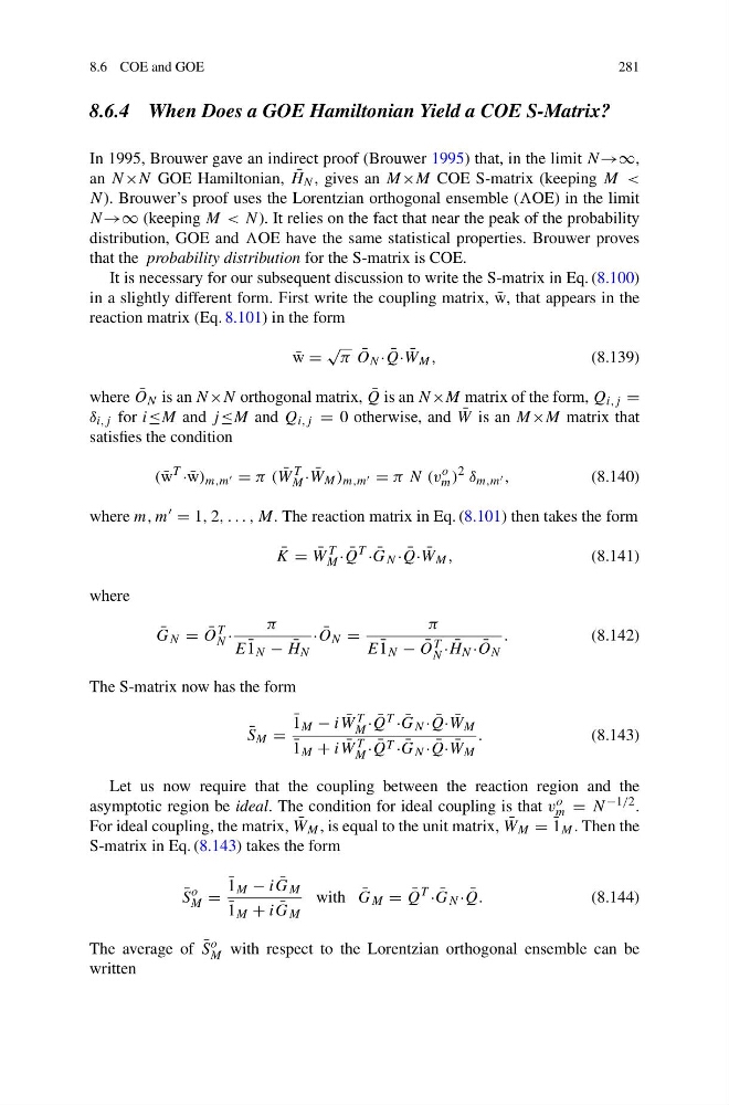
It is necessary for our subsequent discussion to write the S-matrix in Eq. (8.100)
in a slightly different form. First write the coupling matrix, ¯
w, that appears in the
reaction matrix (Eq. 8.101) in the form
¯
w =
√
π ¯
O N · ¯
Q· ¯
W M ,
(8.139)
where ¯
O N is an N×N orthogonal matrix, ¯
Q is an N×M matrix of the form, Q i,j =
δ i,j for i≤M and j ≤M and Q i,j = 0 otherwise, and ¯
W is an M×M matrix that
satisfies the condition
( ¯
w
T
· ¯
w) m,m = π ( ¯
W
T
M · ¯
W M ) m,m = π N (v
o
m )
2 δ m,m ,
(8.140)
where m, m = 1, 2, . . . , M. The reaction matrix in Eq. (8.101) then takes the form
¯
K = ¯
W
T
M · ¯
Q
T
· ¯
G N · ¯
Q· ¯
W M ,
(8.141)
where
¯
G N = ¯
O
T
N ·
π
E ¯
1 N − ¯
H N
· ¯
O N =
π
E ¯
1 N − ¯
O T
N · ¯
H N · ¯
O N
.
(8.142)
The S-matrix now has the form
¯
S M =
¯
1 M − i ¯
W T
M · ¯
Q T · ¯
G N · ¯
Q· ¯
W M
¯
1 M + i ¯
W T
M · ¯
Q T · ¯
G N · ¯
Q· ¯
W M
.
(8.143)
Let us now require that the coupling between the reaction region and the
asymptotic region be ideal. The condition for ideal coupling is that v o
m = N −1/2 .
For ideal coupling, the matrix, ¯
W M , is equal to the unit matrix, ¯
W M = ¯
1 M . Then the
S-matrix in Eq. (8.143) takes the form
¯
S
o
M =
¯
1 M − i ¯
G M
¯
1 M + i ¯
G M
with ¯
G M = ¯
Q
T
· ¯
G N · ¯
Q.
(8.144)
The average of ¯
S o
M with respect to the Lorentzian orthogonal ensemble can be
written
281
8.6.4 When Does a GOE Hamiltonian Yield a COE S-Matrix?
In 1995, Brouwer gave an indirect proof (Brouwer 1995) that, in the limit N→∞,
an N ×N GOE Hamiltonian, ¯
H N , gives an M×M COE S-matrix (keeping M <
N ). Brouwer’s proof uses the Lorentzian orthogonal ensemble (OE) in the limit
N →∞ (keeping M < N). It relies on the fact that near the peak of the probability
distribution, GOE and OE have the same statistical properties. Brouwer proves
that the probability distribution for the S-matrix is COE.
It is necessary for our subsequent discussion to write the S-matrix in Eq. (8.100)
in a slightly different form. First write the coupling matrix, ¯
w, that appears in the
reaction matrix (Eq. 8.101) in the form
¯
w =
√
π ¯
O N · ¯
Q· ¯
W M ,
(8.139)
where ¯
O N is an N×N orthogonal matrix, ¯
Q is an N×M matrix of the form, Q i,j =
δ i,j for i≤M and j ≤M and Q i,j = 0 otherwise, and ¯
W is an M×M matrix that
satisfies the condition
( ¯
w
T
· ¯
w) m,m = π ( ¯
W
T
M · ¯
W M ) m,m = π N (v
o
m )
2 δ m,m ,
(8.140)
where m, m = 1, 2, . . . , M. The reaction matrix in Eq. (8.101) then takes the form
¯
K = ¯
W
T
M · ¯
Q
T
· ¯
G N · ¯
Q· ¯
W M ,
(8.141)
where
¯
G N = ¯
O
T
N ·
π
E ¯
1 N − ¯
H N
· ¯
O N =
π
E ¯
1 N − ¯
O T
N · ¯
H N · ¯
O N
.
(8.142)
The S-matrix now has the form
¯
S M =
¯
1 M − i ¯
W T
M · ¯
Q T · ¯
G N · ¯
Q· ¯
W M
¯
1 M + i ¯
W T
M · ¯
Q T · ¯
G N · ¯
Q· ¯
W M
.
(8.143)
Let us now require that the coupling between the reaction region and the
asymptotic region be ideal. The condition for ideal coupling is that v o
m = N −1/2 .
For ideal coupling, the matrix, ¯
W M , is equal to the unit matrix, ¯
W M = ¯
1 M . Then the
S-matrix in Eq. (8.143) takes the form
¯
S
o
M =
¯
1 M − i ¯
G M
¯
1 M + i ¯
G M
with ¯
G M = ¯
Q
T
· ¯
G N · ¯
Q.
(8.144)
The average of ¯
S o
M with respect to the Lorentzian orthogonal ensemble can be
written