

8.5 Scattering in the Ripple Waveguide
271
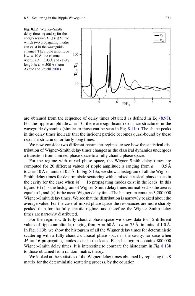
Fig. 8.12 Wigner–Smith
delay times τ 1 and τ 2 for the
energy regime E 1 ≤E≤E 3 for
which two propagating modes
can exist in the waveguide
channel. The ripple amplitude
is a = 10 Å, the channel
width is d = 100 Å and cavity
length is L = 500 Å (from
Akguc and Reichl 2001)
are obtained from the sequence of delay times obtained as defined in Eq. (8.98).
For the ripple amplitude a = 10, there are significant resonance structures in the
waveguide dynamics (similar to those can be seen in Fig. 8.11a). The shape peaks
in the delay times indicate that the incident particle becomes quasi-bound by these
resonant structures for fairly long times.
We now consider two different-parameter regimes to see how the statistical distribution of Wigner–Smith delay times changes as the classical dynamics undergoes
a transition from a mixed phase space to a fully chaotic phase space.
For the regime with mixed phase space, the Wigner–Smith delay times are
computed for 20 different values of ripple amplitude a ranging from a = 0.5 Å
to a = 10 Å in units of 0.5 Å. In Fig. 8.13a, we show a histogram of all the Wigner–
Smith delay times for deterministic scattering with a mixed classical phase space in
the cavity for the case when M = 16 propagating modes exist in the leads. In this
figure, P (τ ) is the histogram of Wigner–Smith delay times normalized so the area is
equal to 1, and is the mean Wigner delay time. The histogram contains 3,200,000
Wigner–Smith delay times. We see that the distribution is narrowly peaked about the
average value. For the case of mixed phase space the resonances are more sharply
peaked than for the fully chaotic regime, and therefore the Wigner–Smith delay
times are narrowly distributed.
For the regime with fully chaotic phase space we show data for 15 different
values of ripple amplitude, ranging from a = 60 Å to a = 75 Å, in units of 1.0 Å.
In Fig. 8.13b, we show the histogram of all the Wigner delay times for deterministic
scattering with a fully chaotic classical phase space in the cavity, for case when
M = 16 propagating modes exist in the leads. Each histogram contains 800,000
Wigner–Smith delay times. It is interesting to compare the histogram in Fig. 8.13b
to those obtained from random matrix theory.
We looked at the statistics of the Wigner delay times obtained by replacing the S
matrix for the deterministic scattering process, by the equation
271
Fig. 8.12 Wigner–Smith
delay times τ 1 and τ 2 for the
energy regime E 1 ≤E≤E 3 for
which two propagating modes
can exist in the waveguide
channel. The ripple amplitude
is a = 10 Å, the channel
width is d = 100 Å and cavity
length is L = 500 Å (from
Akguc and Reichl 2001)
are obtained from the sequence of delay times obtained as defined in Eq. (8.98).
For the ripple amplitude a = 10, there are significant resonance structures in the
waveguide dynamics (similar to those can be seen in Fig. 8.11a). The shape peaks
in the delay times indicate that the incident particle becomes quasi-bound by these
resonant structures for fairly long times.
We now consider two different-parameter regimes to see how the statistical distribution of Wigner–Smith delay times changes as the classical dynamics undergoes
a transition from a mixed phase space to a fully chaotic phase space.
For the regime with mixed phase space, the Wigner–Smith delay times are
computed for 20 different values of ripple amplitude a ranging from a = 0.5 Å
to a = 10 Å in units of 0.5 Å. In Fig. 8.13a, we show a histogram of all the Wigner–
Smith delay times for deterministic scattering with a mixed classical phase space in
the cavity for the case when M = 16 propagating modes exist in the leads. In this
figure, P (τ ) is the histogram of Wigner–Smith delay times normalized so the area is
equal to 1, and is the mean Wigner delay time. The histogram contains 3,200,000
Wigner–Smith delay times. We see that the distribution is narrowly peaked about the
average value. For the case of mixed phase space the resonances are more sharply
peaked than for the fully chaotic regime, and therefore the Wigner–Smith delay
times are narrowly distributed.
For the regime with fully chaotic phase space we show data for 15 different
values of ripple amplitude, ranging from a = 60 Å to a = 75 Å, in units of 1.0 Å.
In Fig. 8.13b, we show the histogram of all the Wigner delay times for deterministic
scattering with a fully chaotic classical phase space in the cavity, for case when
M = 16 propagating modes exist in the leads. Each histogram contains 800,000
Wigner–Smith delay times. It is interesting to compare the histogram in Fig. 8.13b
to those obtained from random matrix theory.
We looked at the statistics of the Wigner delay times obtained by replacing the S
matrix for the deterministic scattering process, by the equation