

8.5 Scattering in the Ripple Waveguide
269
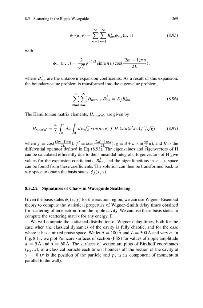
ψ j (u, v) =
∞
m=1
∞
n=1
B
j
mn φ mn (u, v)
(8.95)
with
φ mn (u, v) =
2
√
L
g
−1/2 sin(nπ v) cos(
(2m − 1)π u
2L
),
where B
j
mn are the unknown expansion coefficients. As a result of this expansion,
the boundary value problem is transformed into the eigenvalue problem,
∞
m=1
∞
n=1
H mnm n B
j
mn = E j B
j
mn .
(8.96)
The Hamiltonian matrix elements, H mnm n , are given by
H mnm n =
4
L
L
0
du
1
0
dv
√ g sin(nπv) f ¯
H (sin(n
πv)f
/
√ g)
(8.97)
where f ≡ cos(
(2m−1)π u
2L
), f ≡ cos(
(2m −1)π u
2L
), g ≡ d + a sin(
5π
L u), and ¯
H is the
differential operator defined in Eq. (8.93). The eigenvalues and eigenvectors of H
can be calculated efficiently due to the sinusoidal integrals. Eigenvectors of H give
values for the expansion coefficients, B
j
mn , and the eigenfunctions in u − v space
can be found from these coefficients. The solution can then be transformed back to
x-y space to obtain the basis states, φ j (x, y).
8.5.2.2 Signatures of Chaos in Waveguide Scattering
Given the basis states φ j (x, y) for the reaction region, we can use Wigner–Eisenbud
theory to compute the statistical properties of Wigner–Smith delay times obtained
for scattering of an electron from the ripple cavity. We can use these basis states to
compute the scattering matrix for any energy, E.
We will compute the statistical distribution of Wigner delay times, both for the
case when the classical dynamics of the cavity is fully chaotic, and for the case
where it has a mixed phase space. We let d = 100 Å and L = 500 Å and vary a. In
Fig. 8.11, we plot Poincare surfaces of section (PSS) for values of ripple amplitude
a = 5 Å and a = 60 Å. The surfaces of section are plots of Birkhoff coordinates
(p x , x), of a classical particle each time it bounces off the section of the cavity at
y = 0 (x is the position of the particle and p x is its component of momentum
parallel to the wall).
269
ψ j (u, v) =
∞
m=1
∞
n=1
B
j
mn φ mn (u, v)
(8.95)
with
φ mn (u, v) =
2
√
L
g
−1/2 sin(nπ v) cos(
(2m − 1)π u
2L
),
where B
j
mn are the unknown expansion coefficients. As a result of this expansion,
the boundary value problem is transformed into the eigenvalue problem,
∞
m=1
∞
n=1
H mnm n B
j
mn = E j B
j
mn .
(8.96)
The Hamiltonian matrix elements, H mnm n , are given by
H mnm n =
4
L
L
0
du
1
0
dv
√ g sin(nπv) f ¯
H (sin(n
πv)f
/
√ g)
(8.97)
where f ≡ cos(
(2m−1)π u
2L
), f ≡ cos(
(2m −1)π u
2L
), g ≡ d + a sin(
5π
L u), and ¯
H is the
differential operator defined in Eq. (8.93). The eigenvalues and eigenvectors of H
can be calculated efficiently due to the sinusoidal integrals. Eigenvectors of H give
values for the expansion coefficients, B
j
mn , and the eigenfunctions in u − v space
can be found from these coefficients. The solution can then be transformed back to
x-y space to obtain the basis states, φ j (x, y).
8.5.2.2 Signatures of Chaos in Waveguide Scattering
Given the basis states φ j (x, y) for the reaction region, we can use Wigner–Eisenbud
theory to compute the statistical properties of Wigner–Smith delay times obtained
for scattering of an electron from the ripple cavity. We can use these basis states to
compute the scattering matrix for any energy, E.
We will compute the statistical distribution of Wigner delay times, both for the
case when the classical dynamics of the cavity is fully chaotic, and for the case
where it has a mixed phase space. We let d = 100 Å and L = 500 Å and vary a. In
Fig. 8.11, we plot Poincare surfaces of section (PSS) for values of ripple amplitude
a = 5 Å and a = 60 Å. The surfaces of section are plots of Birkhoff coordinates
(p x , x), of a classical particle each time it bounces off the section of the cavity at
y = 0 (x is the position of the particle and p x is its component of momentum
parallel to the wall).