

268
8 Manifestations of Chaos in Quantum Scattering Processes
8.5.2.1 Basis States for the Reaction Region
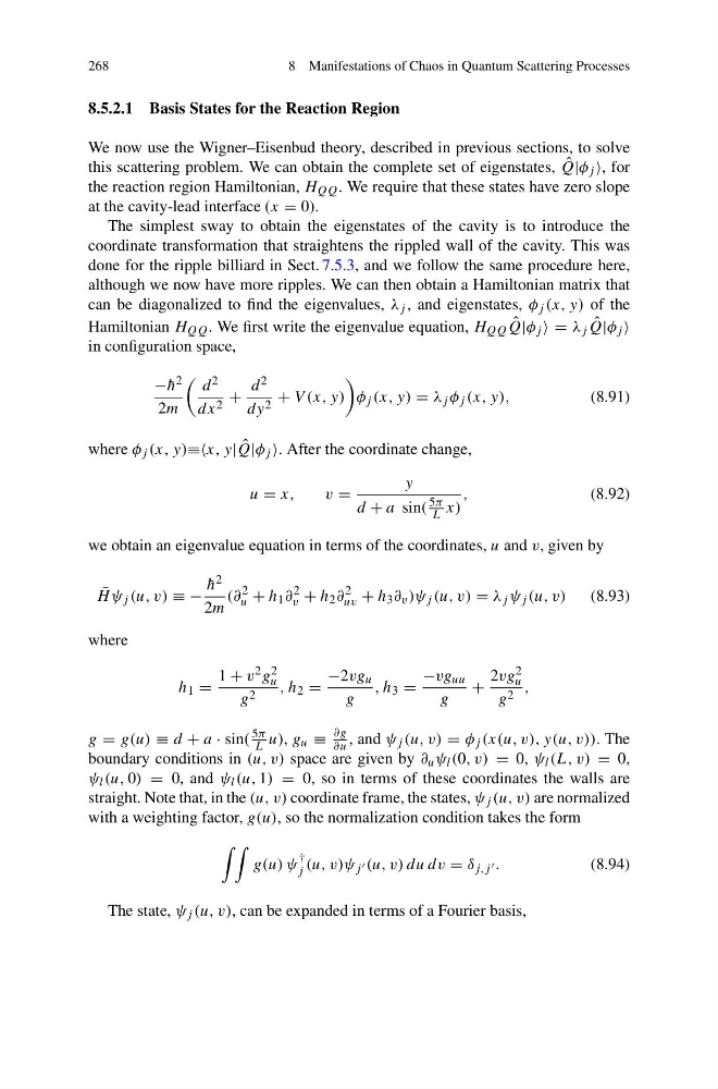
We now use the Wigner–Eisenbud theory, described in previous sections, to solve
this scattering problem. We can obtain the complete set of eigenstates, ˆ
Q|φ j , for
the reaction region Hamiltonian, H QQ . We require that these states have zero slope
at the cavity-lead interface (x = 0).
The simplest sway to obtain the eigenstates of the cavity is to introduce the
coordinate transformation that straightens the rippled wall of the cavity. This was
done for the ripple billiard in Sect. 7.5.3, and we follow the same procedure here,
although we now have more ripples. We can then obtain a Hamiltonian matrix that
can be diagonalized to find the eigenvalues, λ j , and eigenstates, φ j (x, y) of the
Hamiltonian H QQ . We first write the eigenvalue equation, H QQ ˆ
Q|φ j = λ j ˆ
Q|φ j
in configuration space,
− ¯
h 2
2m
d 2
dx 2 +
d 2
dy 2 + V (x, y)
φ j (x, y) = λ j φ j (x, y),
(8.91)
where φ j (x, y)≡≡x, y| ˆ
Q|φ j . After the coordinate change,
u = x,
v =
y
d + a sin(
5π
L x)
,
(8.92)
we obtain an eigenvalue equation in terms of the coordinates, u and v, given by
¯
H ψ j (u, v) ≡ −
¯
h 2
2m
(∂
2
u + h 1 ∂
2
v + h 2 ∂
2
uv + h 3 ∂ v )ψ j (u, v) = λ j ψ j (u, v)
(8.93)
where
h 1 =
1 + v 2 g 2
u
g 2
, h 2 =
−2vg u
g
, h 3 =
−vg uu
g
+
2vg 2
u
g 2 ,
g = g(u) ≡ d + a · sin(
5π
L u), g u ≡
∂g
∂u , and ψ j (u, v) = φ j (x(u, v), y(u, v)). The
boundary conditions in (u, v) space are given by ∂ u ψ l (0, v) = 0, ψ l (L, v) = 0,
ψ l (u, 0) = 0, and ψ l (u, 1) = 0, so in terms of these coordinates the walls are
straight. Note that, in the (u, v) coordinate frame, the states, ψ j (u, v) are normalized
with a weighting factor, g(u), so the normalization condition takes the form
g(u) ψ
†
j (u, v)ψ j (u, v) du dv = δ j,j .
(8.94)
The state, ψ j (u, v), can be expanded in terms of a Fourier basis,
8 Manifestations of Chaos in Quantum Scattering Processes
8.5.2.1 Basis States for the Reaction Region
We now use the Wigner–Eisenbud theory, described in previous sections, to solve
this scattering problem. We can obtain the complete set of eigenstates, ˆ
Q|φ j , for
the reaction region Hamiltonian, H QQ . We require that these states have zero slope
at the cavity-lead interface (x = 0).
The simplest sway to obtain the eigenstates of the cavity is to introduce the
coordinate transformation that straightens the rippled wall of the cavity. This was
done for the ripple billiard in Sect. 7.5.3, and we follow the same procedure here,
although we now have more ripples. We can then obtain a Hamiltonian matrix that
can be diagonalized to find the eigenvalues, λ j , and eigenstates, φ j (x, y) of the
Hamiltonian H QQ . We first write the eigenvalue equation, H QQ ˆ
Q|φ j = λ j ˆ
Q|φ j
in configuration space,
− ¯
h 2
2m
d 2
dx 2 +
d 2
dy 2 + V (x, y)
φ j (x, y) = λ j φ j (x, y),
(8.91)
where φ j (x, y)≡≡x, y| ˆ
Q|φ j . After the coordinate change,
u = x,
v =
y
d + a sin(
5π
L x)
,
(8.92)
we obtain an eigenvalue equation in terms of the coordinates, u and v, given by
¯
H ψ j (u, v) ≡ −
¯
h 2
2m
(∂
2
u + h 1 ∂
2
v + h 2 ∂
2
uv + h 3 ∂ v )ψ j (u, v) = λ j ψ j (u, v)
(8.93)
where
h 1 =
1 + v 2 g 2
u
g 2
, h 2 =
−2vg u
g
, h 3 =
−vg uu
g
+
2vg 2
u
g 2 ,
g = g(u) ≡ d + a · sin(
5π
L u), g u ≡
∂g
∂u , and ψ j (u, v) = φ j (x(u, v), y(u, v)). The
boundary conditions in (u, v) space are given by ∂ u ψ l (0, v) = 0, ψ l (L, v) = 0,
ψ l (u, 0) = 0, and ψ l (u, 1) = 0, so in terms of these coordinates the walls are
straight. Note that, in the (u, v) coordinate frame, the states, ψ j (u, v) are normalized
with a weighting factor, g(u), so the normalization condition takes the form
g(u) ψ
†
j (u, v)ψ j (u, v) du dv = δ j,j .
(8.94)
The state, ψ j (u, v), can be expanded in terms of a Fourier basis,