

14
2 Fundamental Concepts
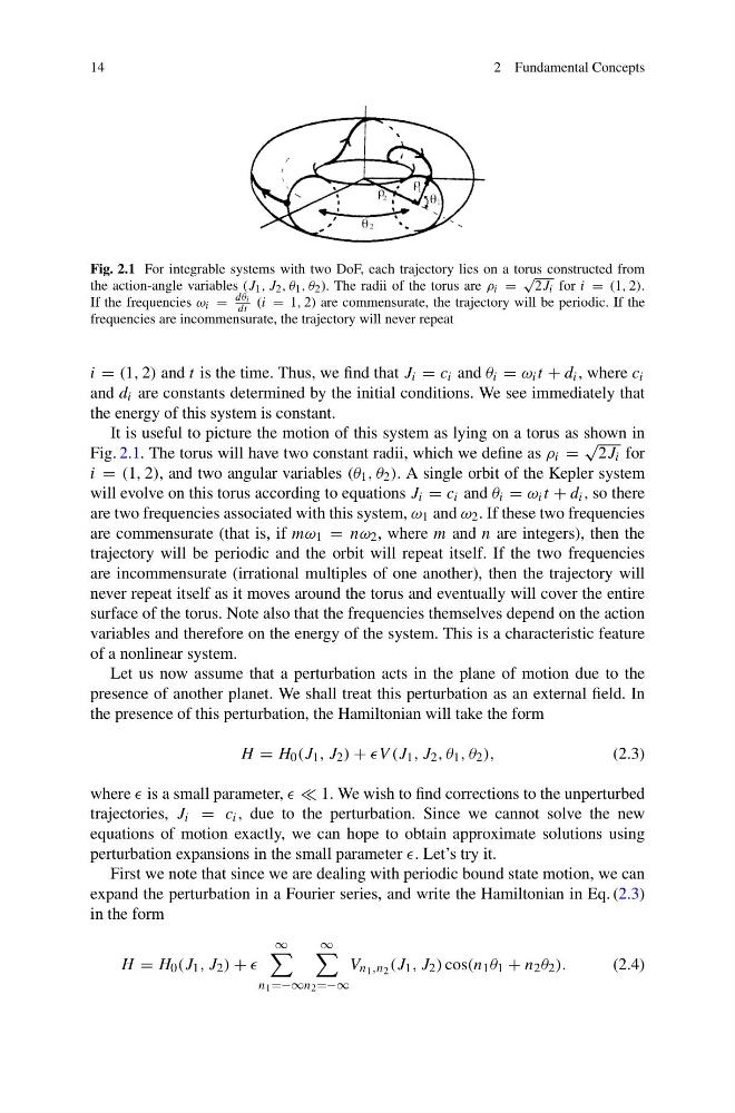
Fig. 2.1 For integrable systems with two DoF, each trajectory lies on a torus constructed from
the action-angle variables (J 1 , J 2 , θ 1 , θ 2 ). The radii of the torus are ρ i =
√
2J i for i = (1, 2).
If the frequencies ω i =
dθ i
dt (i = 1, 2) are commensurate, the trajectory will be periodic. If the
frequencies are incommensurate, the trajectory will never repeat
i = (1, 2) and t is the time. Thus, we find that J i = c i and θ i = ω i t + d i , where c i
and d i are constants determined by the initial conditions. We see immediately that
the energy of this system is constant.
It is useful to picture the motion of this system as lying on a torus as shown in
Fig. 2.1. The torus will have two constant radii, which we define as ρ i =
√
2J i for
i = (1, 2), and two angular variables (θ 1 , θ 2 ). A single orbit of the Kepler system
will evolve on this torus according to equations J i = c i and θ i = ω i t + d i , so there
are two frequencies associated with this system, ω 1 and ω 2 . If these two frequencies
are commensurate (that is, if mω 1 = nω 2 , where m and n are integers), then the
trajectory will be periodic and the orbit will repeat itself. If the two frequencies
are incommensurate (irrational multiples of one another), then the trajectory will
never repeat itself as it moves around the torus and eventually will cover the entire
surface of the torus. Note also that the frequencies themselves depend on the action
variables and therefore on the energy of the system. This is a characteristic feature
of a nonlinear system.
Let us now assume that a perturbation acts in the plane of motion due to the
presence of another planet. We shall treat this perturbation as an external field. In
the presence of this perturbation, the Hamiltonian will take the form
H = H 0 (J 1 , J 2 ) + (J 1 , J 2 , θ 1 , θ 2 ),
(2.3)
where is a small parameter, 1. We wish to find corrections to the unperturbed
trajectories, J i = c i , due to the perturbation. Since we cannot solve the new
equations of motion exactly, we can hope to obtain approximate solutions using
perturbation expansions in the small parameter . Let’s try it.
First we note that since we are dealing with periodic bound state motion, we can
expand the perturbation in a Fourier series, and write the Hamiltonian in Eq. (2.3)
in the form
H = H 0 (J 1 , J 2 ) +
∞
n 1 =−∞
∞
n 2 =−∞
V n 1 ,n 2 (J 1 , J 2 ) cos(n 1 θ 1 + n 2 θ 2 ).
(2.4)
2 Fundamental Concepts
Fig. 2.1 For integrable systems with two DoF, each trajectory lies on a torus constructed from
the action-angle variables (J 1 , J 2 , θ 1 , θ 2 ). The radii of the torus are ρ i =
√
2J i for i = (1, 2).
If the frequencies ω i =
dθ i
dt (i = 1, 2) are commensurate, the trajectory will be periodic. If the
frequencies are incommensurate, the trajectory will never repeat
i = (1, 2) and t is the time. Thus, we find that J i = c i and θ i = ω i t + d i , where c i
and d i are constants determined by the initial conditions. We see immediately that
the energy of this system is constant.
It is useful to picture the motion of this system as lying on a torus as shown in
Fig. 2.1. The torus will have two constant radii, which we define as ρ i =
√
2J i for
i = (1, 2), and two angular variables (θ 1 , θ 2 ). A single orbit of the Kepler system
will evolve on this torus according to equations J i = c i and θ i = ω i t + d i , so there
are two frequencies associated with this system, ω 1 and ω 2 . If these two frequencies
are commensurate (that is, if mω 1 = nω 2 , where m and n are integers), then the
trajectory will be periodic and the orbit will repeat itself. If the two frequencies
are incommensurate (irrational multiples of one another), then the trajectory will
never repeat itself as it moves around the torus and eventually will cover the entire
surface of the torus. Note also that the frequencies themselves depend on the action
variables and therefore on the energy of the system. This is a characteristic feature
of a nonlinear system.
Let us now assume that a perturbation acts in the plane of motion due to the
presence of another planet. We shall treat this perturbation as an external field. In
the presence of this perturbation, the Hamiltonian will take the form
H = H 0 (J 1 , J 2 ) + (J 1 , J 2 , θ 1 , θ 2 ),
(2.3)
where is a small parameter, 1. We wish to find corrections to the unperturbed
trajectories, J i = c i , due to the perturbation. Since we cannot solve the new
equations of motion exactly, we can hope to obtain approximate solutions using
perturbation expansions in the small parameter . Let’s try it.
First we note that since we are dealing with periodic bound state motion, we can
expand the perturbation in a Fourier series, and write the Hamiltonian in Eq. (2.3)
in the form
H = H 0 (J 1 , J 2 ) +
∞
n 1 =−∞
∞
n 2 =−∞
V n 1 ,n 2 (J 1 , J 2 ) cos(n 1 θ 1 + n 2 θ 2 ).
(2.4)