

2.2 Conventional Perturbation Theory
15
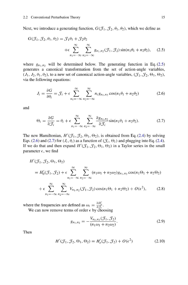
Next, we introduce a generating function, G(J 1 , J 2 , θ 1 , θ 2 ), which we define as
G(J 1 , J 2 , θ 1 , θ 2 ) = J 1 θ 1 + J 2 θ 2
+
∞
n 1 =−∞
∞
n 2 =−∞
g n 1 ,n 2 (J 1 , J 2 ) sin(n 1 θ 1 + n 2 θ 2 ), (2.5)
where g n 1 ,n 2 will be determined below. The generating function in Eq. (2.5)
generates a canonical transformation from the set of action-angle variables,
(J 1 , J 2 , θ 1 , θ 2 ), to a new set of canonical action-angle variables, (J 1 , J 2 , , 1 , , 2 ),
via the following equations:
J i =
∂G
∂θ i
= J i +
∞
n 1 =−∞
∞
n 2 =−∞
n i g n 1 ,n 2 cos(n 1 θ 1 + n 2 θ 2 )
(2.6)
and
i =
∂G
∂J i
= θ i +
∞
n 1 =−∞
∞
n 2 =−∞
∂g n 1 ,n 2
∂J i
sin(n 1 θ 1 + n 2 θ 2 ).
(2.7)
The new Hamiltonian, H (J 1 , J 2 , , 1 , , 2 ), is obtained from Eq. (2.4) by solving
Eqs. (2.6) and (2.7) for (J i , θ i ) as a function of (J i , , i ) and plugging into Eq. (2.4).
If we do that and then expand H (J 1 , J 2 , , 1 , , 2 ) in a Taylor series in the small
parameter , we find
H
(J 1 , J 2 , , 1 , , 2 )
= H
0 (J 1 , J 2 ) +
∞
n 1 =−∞
∞
n 2 =−∞
(n 1 ω 1 + n 2 ω 2 )g n 1 ,n 2 cos(n 1 1 + n 2 2 )
+
∞
n 1 =−∞
∞
n 2 =−∞
V n 1 ,n 2 (J 1 , J 2 ) cos(n 1 1 + n 2 2 ) + O((
2 ),
(2.8)
where the frequencies are defined as ω i =
∂H
o
∂J i
.
We can now remove terms of order by choosing
g n 1 ,n 2 = −
V n 1 ,n 2 (J 1 , J 2 )
(n 1 ω 1 + n 2 ω 2 )
.
(2.9)
Then
H
(J 1 , J 2 , , 1 , , 2 ) = H
o (J 1 , J 2 ) + O((
2 )
(2.10)
15
Next, we introduce a generating function, G(J 1 , J 2 , θ 1 , θ 2 ), which we define as
G(J 1 , J 2 , θ 1 , θ 2 ) = J 1 θ 1 + J 2 θ 2
+
∞
n 1 =−∞
∞
n 2 =−∞
g n 1 ,n 2 (J 1 , J 2 ) sin(n 1 θ 1 + n 2 θ 2 ), (2.5)
where g n 1 ,n 2 will be determined below. The generating function in Eq. (2.5)
generates a canonical transformation from the set of action-angle variables,
(J 1 , J 2 , θ 1 , θ 2 ), to a new set of canonical action-angle variables, (J 1 , J 2 , , 1 , , 2 ),
via the following equations:
J i =
∂G
∂θ i
= J i +
∞
n 1 =−∞
∞
n 2 =−∞
n i g n 1 ,n 2 cos(n 1 θ 1 + n 2 θ 2 )
(2.6)
and
i =
∂G
∂J i
= θ i +
∞
n 1 =−∞
∞
n 2 =−∞
∂g n 1 ,n 2
∂J i
sin(n 1 θ 1 + n 2 θ 2 ).
(2.7)
The new Hamiltonian, H (J 1 , J 2 , , 1 , , 2 ), is obtained from Eq. (2.4) by solving
Eqs. (2.6) and (2.7) for (J i , θ i ) as a function of (J i , , i ) and plugging into Eq. (2.4).
If we do that and then expand H (J 1 , J 2 , , 1 , , 2 ) in a Taylor series in the small
parameter , we find
H
(J 1 , J 2 , , 1 , , 2 )
= H
0 (J 1 , J 2 ) +
∞
n 1 =−∞
∞
n 2 =−∞
(n 1 ω 1 + n 2 ω 2 )g n 1 ,n 2 cos(n 1 1 + n 2 2 )
+
∞
n 1 =−∞
∞
n 2 =−∞
V n 1 ,n 2 (J 1 , J 2 ) cos(n 1 1 + n 2 2 ) + O((
2 ),
(2.8)
where the frequencies are defined as ω i =
∂H
o
∂J i
.
We can now remove terms of order by choosing
g n 1 ,n 2 = −
V n 1 ,n 2 (J 1 , J 2 )
(n 1 ω 1 + n 2 ω 2 )
.
(2.9)
Then
H
(J 1 , J 2 , , 1 , , 2 ) = H
o (J 1 , J 2 ) + O((
2 )
(2.10)