

2.2 Conventional Perturbation Theory
13
In practice, chaos is defined in terms of the dynamical behavior of pairs of
orbits that initially are close together in the phase space. If the orbits move apart
exponentially in any direction in the phase space, the flow is said to be chaotic.
The rate of exponential divergence of pairs of orbits is measured by the so-called
Lyapounov exponents. There will be one such exponent for each dimension in the
phase space. If all the Lyapounov exponents are zero, the dynamical flow is regular.
If even one exponent is positive, the flow will be chaotic. A detailed discussion of the
behavior of Lyapounov exponents for conservative systems is given in Sect. 2.7 and
is illustrated in terms of the Henon-Heiles system. Systems with positive Lyapounov
exponents also have positive KS metric entropy. The KS metric entropy is defined
in Sect. 2.7 and computed for the baker’s transformation, one of the simplest known
chaotic dynamical systems.
Finally, in Sect. 2.8, we make some concluding remarks.
2.2 Conventional Perturbation Theory
Historically the first cracks in a deterministic view of the world, and an appreciation
of the difficulties in obtaining long-time predictions regarding the evolution of
dynamical systems, were brought into focus with Poincaré’s proof that conventional
perturbation expansions generally diverge. When they diverge they cannot be used
as a tool to provide long-time predictions.
In order to build some intuition concerning the origin of these divergences, let us
consider a 2 DoF system from celestial mechanics, the relative motion of a moon of
mass m 1 , orbiting a planet of mass m 2 (the Kepler system). The Hamiltonian can be
written
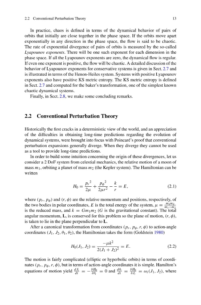
H 0 =
p r
2
2μ
+
p φ
2
2μr 2 −
k
r
= E,
(2.1)
where (p r , p φ ) and (r, φ) are the relative momentum and positions, respectively, of
the two bodies in polar coordinates, E is the total energy of the system, μ =
m 1 m 2
m 1 +m 2
is the reduced mass, and k = Gm 1 m 2 (G is the gravitational constant). The total
angular momentum, L, is conserved for this problem so the plane of motion, (r, φ),
is taken to lie in the plane perpendicular to L.
After a canonical transformation from coordinates (p r , p φ , r, φ) to action-angle
coordinates (J 1 , J 2 , θ 1 , θ 2 ), the Hamiltonian takes the form (Goldstein 1980)
H 0 (J 1 , J 2 ) =
−μk 2
2(J 1 + J 2 ) 2 = E.
(2.2)
The motion is fairly complicated (elliptic or hyperbolic orbits) in terms of coordinates (p r , p φ , r, φ), but in terms of action-angle coordinates it is simple. Hamilton’s
equations of motion yield
dJ i
dt = −
∂H 0
∂θ i
= 0 and
dθ i
dt =
∂H 0
∂J i
= ω i (J 1 , J 2 ), where
13
In practice, chaos is defined in terms of the dynamical behavior of pairs of
orbits that initially are close together in the phase space. If the orbits move apart
exponentially in any direction in the phase space, the flow is said to be chaotic.
The rate of exponential divergence of pairs of orbits is measured by the so-called
Lyapounov exponents. There will be one such exponent for each dimension in the
phase space. If all the Lyapounov exponents are zero, the dynamical flow is regular.
If even one exponent is positive, the flow will be chaotic. A detailed discussion of the
behavior of Lyapounov exponents for conservative systems is given in Sect. 2.7 and
is illustrated in terms of the Henon-Heiles system. Systems with positive Lyapounov
exponents also have positive KS metric entropy. The KS metric entropy is defined
in Sect. 2.7 and computed for the baker’s transformation, one of the simplest known
chaotic dynamical systems.
Finally, in Sect. 2.8, we make some concluding remarks.
2.2 Conventional Perturbation Theory
Historically the first cracks in a deterministic view of the world, and an appreciation
of the difficulties in obtaining long-time predictions regarding the evolution of
dynamical systems, were brought into focus with Poincaré’s proof that conventional
perturbation expansions generally diverge. When they diverge they cannot be used
as a tool to provide long-time predictions.
In order to build some intuition concerning the origin of these divergences, let us
consider a 2 DoF system from celestial mechanics, the relative motion of a moon of
mass m 1 , orbiting a planet of mass m 2 (the Kepler system). The Hamiltonian can be
written
H 0 =
p r
2
2μ
+
p φ
2
2μr 2 −
k
r
= E,
(2.1)
where (p r , p φ ) and (r, φ) are the relative momentum and positions, respectively, of
the two bodies in polar coordinates, E is the total energy of the system, μ =
m 1 m 2
m 1 +m 2
is the reduced mass, and k = Gm 1 m 2 (G is the gravitational constant). The total
angular momentum, L, is conserved for this problem so the plane of motion, (r, φ),
is taken to lie in the plane perpendicular to L.
After a canonical transformation from coordinates (p r , p φ , r, φ) to action-angle
coordinates (J 1 , J 2 , θ 1 , θ 2 ), the Hamiltonian takes the form (Goldstein 1980)
H 0 (J 1 , J 2 ) =
−μk 2
2(J 1 + J 2 ) 2 = E.
(2.2)
The motion is fairly complicated (elliptic or hyperbolic orbits) in terms of coordinates (p r , p φ , r, φ), but in terms of action-angle coordinates it is simple. Hamilton’s
equations of motion yield
dJ i
dt = −
∂H 0
∂θ i
= 0 and
dθ i
dt =
∂H 0
∂J i
= ω i (J 1 , J 2 ), where