

8.3 Scattering Theory
251
R(E) =
2
a 2
∞
j =1
1
k 2 − κ 2 −
π 2 (2j −1) 2
4a 2
≡
tan(
√
k 2 − κ 2 a)
√
k 2 − κ 2 a
.
(8.33)
In this case, the reaction function is just the series expansion for the function
tan(
√
k 2 −κ 2 a)
√
k 2 −κ 2 a
(Reichl and Akguc 2001).
8.3.4 The Scattering Matrix
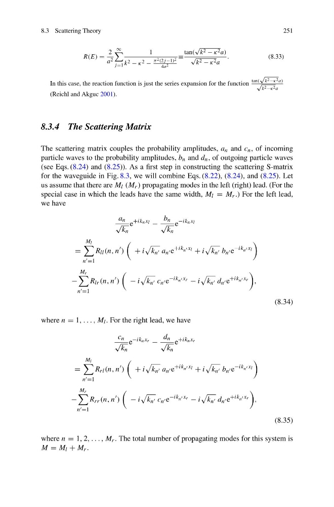
The scattering matrix couples the probability amplitudes, a n and c n , of incoming
particle waves to the probability amplitudes, b n and d n , of outgoing particle waves
(see Eqs. (8.24) and (8.25)). As a first step in constructing the scattering S-matrix
for the waveguide in Fig. 8.3, we will combine Eqs. (8.22), (8.24), and (8.25). Let
us assume that there are M l (M r ) propagating modes in the left (right) lead. (For the
special case in which the leads have the same width, M l = M r .) For the left lead,
we have
a n
√
k n
e
+ik n x l −
b n
√
k n
e
−ik n x l
=
M l
n =1
R ll (n, n
)
+ i
k n a n e
+ik n x l + i
k n b n e
−ik n x l
−
M r
n =1
R lr (n, n
)
− i
k n c n e
−ik n x r − i
k n d n e
+ik n x r
,
(8.34)
where n = 1, . . . , M l . For the right lead, we have
c n
√
k n
e
−ik n x r −
d n
√
k n
e
+ik n x r
=
M l
n =1
R rl (n, n
)
+ i
k n a n e
+ik n x l + i
k n b n e
−ik n x l
−
M r
n =1
R rr (n, n
)
− i
k n c n e
−ik n x r − i
k n d n e
+ik n x r
,
(8.35)
where n = 1, 2, . . . , M r . The total number of propagating modes for this system is
M = M l + M r .
251
R(E) =
2
a 2
∞
j =1
1
k 2 − κ 2 −
π 2 (2j −1) 2
4a 2
≡
tan(
√
k 2 − κ 2 a)
√
k 2 − κ 2 a
.
(8.33)
In this case, the reaction function is just the series expansion for the function
tan(
√
k 2 −κ 2 a)
√
k 2 −κ 2 a
(Reichl and Akguc 2001).
8.3.4 The Scattering Matrix
The scattering matrix couples the probability amplitudes, a n and c n , of incoming
particle waves to the probability amplitudes, b n and d n , of outgoing particle waves
(see Eqs. (8.24) and (8.25)). As a first step in constructing the scattering S-matrix
for the waveguide in Fig. 8.3, we will combine Eqs. (8.22), (8.24), and (8.25). Let
us assume that there are M l (M r ) propagating modes in the left (right) lead. (For the
special case in which the leads have the same width, M l = M r .) For the left lead,
we have
a n
√
k n
e
+ik n x l −
b n
√
k n
e
−ik n x l
=
M l
n =1
R ll (n, n
)
+ i
k n a n e
+ik n x l + i
k n b n e
−ik n x l
−
M r
n =1
R lr (n, n
)
− i
k n c n e
−ik n x r − i
k n d n e
+ik n x r
,
(8.34)
where n = 1, . . . , M l . For the right lead, we have
c n
√
k n
e
−ik n x r −
d n
√
k n
e
+ik n x r
=
M l
n =1
R rl (n, n
)
+ i
k n a n e
+ik n x l + i
k n b n e
−ik n x l
−
M r
n =1
R rr (n, n
)
− i
k n c n e
−ik n x r − i
k n d n e
+ik n x r
,
(8.35)
where n = 1, 2, . . . , M r . The total number of propagating modes for this system is
M = M l + M r .