

252
8 Manifestations of Chaos in Quantum Scattering Processes
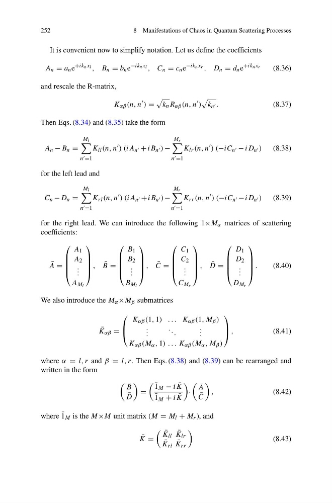
It is convenient now to simplify notation. Let us define the coefficients
A n = a n e
+ik n x l , B n = b n e
−ik n x l , C n = c n e
−ik n x r , D n = d n e
+ik n x r
(8.36)
and rescale the R-matrix,
K αβ (n, n
) =
k n R αβ (n, n
)
k n .
(8.37)
Then Eqs. (8.34) and (8.35) take the form
A n − B n =
M l
n =1
K ll (n, n
) (iA n + iB n ) −
M r
n =1
K lr (n, n
) (−iC n − iD n ) (8.38)
for the left lead and
C n − D n =
M l
n =1
K rl (n, n
) (iA n + iB n ) −
M r
n =1
K rr (n, n
) (−iC n − iD n ) (8.39)
for the right lead. We can introduce the following 1×M α matrices of scattering
coefficients:
¯
A =
⎛
⎜
⎜
⎜
⎝
A 1
A 2
. . .
A M l
⎞
⎟
⎟
⎟
⎠
, ¯
B =
⎛
⎜
⎜
⎜
⎝
B 1
B 2
. . .
B M l
⎞
⎟
⎟
⎟
⎠
, ¯
C =
⎛
⎜
⎜
⎜
⎝
C 1
C 2
. . .
C M r
⎞
⎟
⎟
⎟
⎠
, ¯
D =
⎛
⎜
⎜
⎜
⎝
D 1
D 2
. . .
D M r
⎞
⎟
⎟
⎟
⎠
.
(8.40)
We also introduce the M α ×M β submatrices
¯
K αβ =
⎛
⎜
⎝
K αβ (1, 1) ... K αβ (1, M β )
. . .
. . .
. . .
K αβ (M α , 1) . . . K αβ (M α , M β )
⎞
⎟
⎠ ,
(8.41)
where α = l, r and β = l, r. Then Eqs. (8.38) and (8.39) can be rearranged and
written in the form
¯
B
¯
D
=
¯
1 M − i ¯
K
¯
1 M + i ¯
K
·
¯
A
¯
C
,
(8.42)
where ¯
1 M is the M×M unit matrix (M = M l + M r ), and
¯
K =
¯
K ll ¯
K lr
¯
K rl ¯
K rr
(8.43)
8 Manifestations of Chaos in Quantum Scattering Processes
It is convenient now to simplify notation. Let us define the coefficients
A n = a n e
+ik n x l , B n = b n e
−ik n x l , C n = c n e
−ik n x r , D n = d n e
+ik n x r
(8.36)
and rescale the R-matrix,
K αβ (n, n
) =
k n R αβ (n, n
)
k n .
(8.37)
Then Eqs. (8.34) and (8.35) take the form
A n − B n =
M l
n =1
K ll (n, n
) (iA n + iB n ) −
M r
n =1
K lr (n, n
) (−iC n − iD n ) (8.38)
for the left lead and
C n − D n =
M l
n =1
K rl (n, n
) (iA n + iB n ) −
M r
n =1
K rr (n, n
) (−iC n − iD n ) (8.39)
for the right lead. We can introduce the following 1×M α matrices of scattering
coefficients:
¯
A =
⎛
⎜
⎜
⎜
⎝
A 1
A 2
. . .
A M l
⎞
⎟
⎟
⎟
⎠
, ¯
B =
⎛
⎜
⎜
⎜
⎝
B 1
B 2
. . .
B M l
⎞
⎟
⎟
⎟
⎠
, ¯
C =
⎛
⎜
⎜
⎜
⎝
C 1
C 2
. . .
C M r
⎞
⎟
⎟
⎟
⎠
, ¯
D =
⎛
⎜
⎜
⎜
⎝
D 1
D 2
. . .
D M r
⎞
⎟
⎟
⎟
⎠
.
(8.40)
We also introduce the M α ×M β submatrices
¯
K αβ =
⎛
⎜
⎝
K αβ (1, 1) ... K αβ (1, M β )
. . .
. . .
. . .
K αβ (M α , 1) . . . K αβ (M α , M β )
⎞
⎟
⎠ ,
(8.41)
where α = l, r and β = l, r. Then Eqs. (8.38) and (8.39) can be rearranged and
written in the form
¯
B
¯
D
=
¯
1 M − i ¯
K
¯
1 M + i ¯
K
·
¯
A
¯
C
,
(8.42)
where ¯
1 M is the M×M unit matrix (M = M l + M r ), and
¯
K =
¯
K ll ¯
K lr
¯
K rl ¯
K rr
(8.43)