

6.5 Eigenvector Statistics: Gaussian Orthogonal Ensemble
185
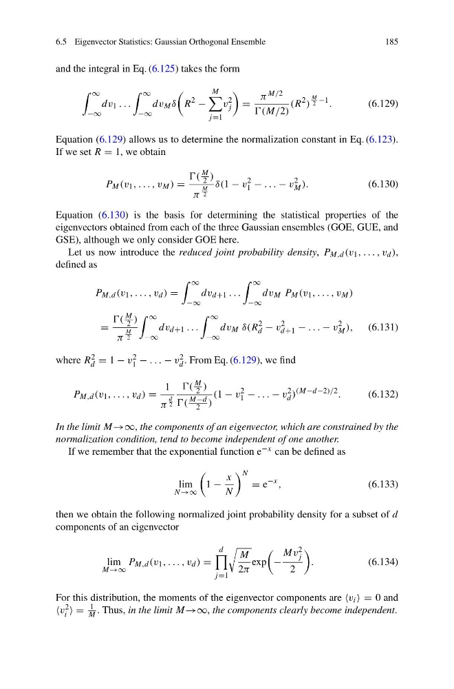
and the integral in Eq. (6.125) takes the form
∞
−∞
dv 1 . . .
∞
−∞
dv M δ
R
2
−
M
j =1
v
2
j
=
π M/2
(M/2)
(R
2 )
M
2 −1 .
(6.129)
Equation (6.129) allows us to determine the normalization constant in Eq. (6.123).
If we set R = 1, we obtain
P M (v 1 , . . . , v M ) =
(
M
2 )
π
M
2
δ(1 − v
2
1 − . . . − v
2
M ).
(6.130)
Equation (6.130) is the basis for determining the statistical properties of the
eigenvectors obtained from each of the three Gaussian ensembles (GOE, GUE, and
GSE), although we only consider GOE here.
Let us now introduce the reduced joint probability density, P M,d (v 1 , . . . , v d ),
defined as
P M,d (v 1 , . . . , v d ) =
∞
−∞
dv d+1 . . .
∞
−∞
dv M P M (v 1 , . . . , v M )
=
(
M
2 )
π
M
2
∞
−∞
dv d+1 . . .
∞
−∞
dv M δ(R
2
d − v
2
d+1 − . . . − v
2
M ), (6.131)
where R 2
d = 1 − v 2
1 − . . . − v 2
d . From Eq. (6.129), we find
P M,d (v 1 , . . . , v d ) =
1
π
d
2
(
M
2 )
(
M−d
2 )
(1 − v
2
1 − . . . − v
2
d )
(M−d−2)/2 .
(6.132)
In the limit M→∞, the components of an eigenvector, which are constrained by the
normalization condition, tend to become independent of one another.
If we remember that the exponential function e −x can be defined as
lim
N →∞
1 −
x
N
N
= e
−x ,
(6.133)
then we obtain the following normalized joint probability density for a subset of d
components of an eigenvector
lim
M→∞
P M,d (v 1 , . . . , v d ) =
d
j =1
M
2π
exp
−
Mv 2
j
2
.
(6.134)
For this distribution, the moments of the eigenvector components are v i = 0 and
v 2
i =
1
M . Thus, in the limit M→∞, the components clearly become independent.
185
and the integral in Eq. (6.125) takes the form
∞
−∞
dv 1 . . .
∞
−∞
dv M δ
R
2
−
M
j =1
v
2
j
=
π M/2
(M/2)
(R
2 )
M
2 −1 .
(6.129)
Equation (6.129) allows us to determine the normalization constant in Eq. (6.123).
If we set R = 1, we obtain
P M (v 1 , . . . , v M ) =
(
M
2 )
π
M
2
δ(1 − v
2
1 − . . . − v
2
M ).
(6.130)
Equation (6.130) is the basis for determining the statistical properties of the
eigenvectors obtained from each of the three Gaussian ensembles (GOE, GUE, and
GSE), although we only consider GOE here.
Let us now introduce the reduced joint probability density, P M,d (v 1 , . . . , v d ),
defined as
P M,d (v 1 , . . . , v d ) =
∞
−∞
dv d+1 . . .
∞
−∞
dv M P M (v 1 , . . . , v M )
=
(
M
2 )
π
M
2
∞
−∞
dv d+1 . . .
∞
−∞
dv M δ(R
2
d − v
2
d+1 − . . . − v
2
M ), (6.131)
where R 2
d = 1 − v 2
1 − . . . − v 2
d . From Eq. (6.129), we find
P M,d (v 1 , . . . , v d ) =
1
π
d
2
(
M
2 )
(
M−d
2 )
(1 − v
2
1 − . . . − v
2
d )
(M−d−2)/2 .
(6.132)
In the limit M→∞, the components of an eigenvector, which are constrained by the
normalization condition, tend to become independent of one another.
If we remember that the exponential function e −x can be defined as
lim
N →∞
1 −
x
N
N
= e
−x ,
(6.133)
then we obtain the following normalized joint probability density for a subset of d
components of an eigenvector
lim
M→∞
P M,d (v 1 , . . . , v d ) =
d
j =1
M
2π
exp
−
Mv 2
j
2
.
(6.134)
For this distribution, the moments of the eigenvector components are v i = 0 and
v 2
i =
1
M . Thus, in the limit M→∞, the components clearly become independent.