

186
6 Quantum Dynamics and Random Matrix Theory
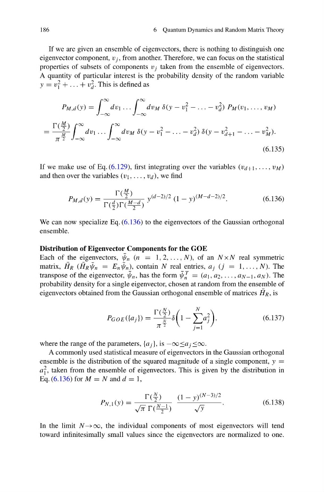
If we are given an ensemble of eigenvectors, there is nothing to distinguish one
eigenvector component, v j , from another. Therefore, we can focus on the statistical
properties of subsets of components v j taken from the ensemble of eigenvectors.
A quantity of particular interest is the probability density of the random variable
y = v 2
1 + . . . + v 2
d . This is defined as
P M,d (y) =
∞
−∞
dv 1 . . .
∞
−∞
dv M δ(y − v
2
1 − . . . − v
2
d ) P M (v 1 , . . . , v M )
=
(
M
2 )
π
M
2
∞
−∞
dv 1 . . .
∞
−∞
dv M δ(y − v
2
1 − . . . − v
2
d ) δ(y − v
2
d+1 − . . . − v
2
M ).
(6.135)
If we make use of Eq. (6.129), first integrating over the variables (v d+1 , . . . , v M )
and then over the variables (v 1 , . . . , v d ), we find
P M,d (y) =
(
M
2 )
(
d
2 ))(
M−d
2 )
y
(d−2)/2 (1 − y)
(M−d−2)/2 .
(6.136)
We can now specialize Eq. (6.136) to the eigenvectors of the Gaussian orthogonal
ensemble.
Distribution of Eigenvector Components for the GOE
Each of the eigenvectors, ¯
ψ n (n = 1, 2, . . . , N), of an N×N real symmetric
matrix, ¯
H R ( ¯
H R ¯
ψ n = E n ¯
ψ n ), contain N real entries, a j (j = 1, . . . , N). The
transpose of the eigenvector, ¯
ψ n , has the form ¯
ψ T
n = (a 1 , a 2 , . . . , a N −1 , a N ). The
probability density for a single eigenvector, chosen at random from the ensemble of
eigenvectors obtained from the Gaussian orthogonal ensemble of matrices ¯
H R , is
P GOE ({a j }) =
(
N
2 )
π
N
2
δ
1 −
N
j =1
a
2
j
,
(6.137)
where the range of the parameters, {a j }, is −∞≤a j ≤∞.
A commonly used statistical measure of eigenvectors in the Gaussian orthogonal
ensemble is the distribution of the squared magnitude of a single component, y =
a 2
1 , taken from the ensemble of eigenvectors. This is given by the distribution in
Eq. (6.136) for M = N and d = 1,
P N,1 (y) =
(
N
2 )
√
π π(
N −1
2 )
(1 − y) (N −3)/2
√ y
.
(6.138)
In the limit N →∞, the individual components of most eigenvectors will tend
toward infinitesimally small values since the eigenvectors are normalized to one.
6 Quantum Dynamics and Random Matrix Theory
If we are given an ensemble of eigenvectors, there is nothing to distinguish one
eigenvector component, v j , from another. Therefore, we can focus on the statistical
properties of subsets of components v j taken from the ensemble of eigenvectors.
A quantity of particular interest is the probability density of the random variable
y = v 2
1 + . . . + v 2
d . This is defined as
P M,d (y) =
∞
−∞
dv 1 . . .
∞
−∞
dv M δ(y − v
2
1 − . . . − v
2
d ) P M (v 1 , . . . , v M )
=
(
M
2 )
π
M
2
∞
−∞
dv 1 . . .
∞
−∞
dv M δ(y − v
2
1 − . . . − v
2
d ) δ(y − v
2
d+1 − . . . − v
2
M ).
(6.135)
If we make use of Eq. (6.129), first integrating over the variables (v d+1 , . . . , v M )
and then over the variables (v 1 , . . . , v d ), we find
P M,d (y) =
(
M
2 )
(
d
2 ))(
M−d
2 )
y
(d−2)/2 (1 − y)
(M−d−2)/2 .
(6.136)
We can now specialize Eq. (6.136) to the eigenvectors of the Gaussian orthogonal
ensemble.
Distribution of Eigenvector Components for the GOE
Each of the eigenvectors, ¯
ψ n (n = 1, 2, . . . , N), of an N×N real symmetric
matrix, ¯
H R ( ¯
H R ¯
ψ n = E n ¯
ψ n ), contain N real entries, a j (j = 1, . . . , N). The
transpose of the eigenvector, ¯
ψ n , has the form ¯
ψ T
n = (a 1 , a 2 , . . . , a N −1 , a N ). The
probability density for a single eigenvector, chosen at random from the ensemble of
eigenvectors obtained from the Gaussian orthogonal ensemble of matrices ¯
H R , is
P GOE ({a j }) =
(
N
2 )
π
N
2
δ
1 −
N
j =1
a
2
j
,
(6.137)
where the range of the parameters, {a j }, is −∞≤a j ≤∞.
A commonly used statistical measure of eigenvectors in the Gaussian orthogonal
ensemble is the distribution of the squared magnitude of a single component, y =
a 2
1 , taken from the ensemble of eigenvectors. This is given by the distribution in
Eq. (6.136) for M = N and d = 1,
P N,1 (y) =
(
N
2 )
√
π π(
N −1
2 )
(1 − y) (N −3)/2
√ y
.
(6.138)
In the limit N →∞, the individual components of most eigenvectors will tend
toward infinitesimally small values since the eigenvectors are normalized to one.