

6.4 Eigenvalue Statistics: Gaussian Orthogonal Ensemble
181
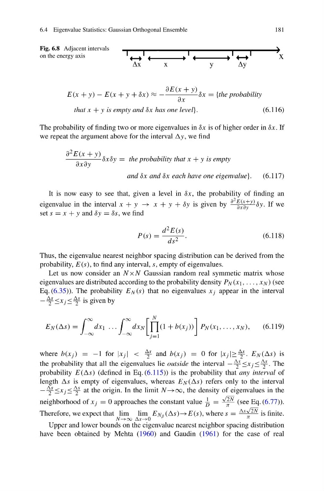
Fig. 6.8 Adjacent intervals
on the energy axis
E(x + y) − E(x + y + δx) ≈ −
∂E(x + y)
∂x
δx = {the probability
that x + y is empty and δx has one level}.
(6.116)
The probability of finding two or more eigenvalues in δx is of higher order in δx. If
we repeat the argument above for the interval y, we find
∂ 2 E(x + y)
∂x∂y
δxδy = the probability that x + y is empty
and δx and δx each have one eigenvalue}. (6.117)
It is now easy to see that, given a level in δx, the probability of finding an
eigenvalue in the interval x + y → x + y + δy is given by
∂ 2 E(x+y)
∂x∂y δy. If we
set s = x + y and δy = δs, we find
P (s) =
d 2 E(s)
ds 2 .
(6.118)
Thus, the eigenvalue nearest neighbor spacing distribution can be derived from the
probability, E(s), to find any interval, s, empty of eigenvalues.
Let us now consider an N ×N Gaussian random real symmetic matrix whose
eigenvalues are distributed according to the probability density P N (x 1 , . . . , x N ) (see
Eq. (6.35)). The probability E N (s) that no eigenvalues x j appear in the interval
−
2 ≤x j ≤
2 is given by
E N ((s) =
∞
−∞
dx 1 . . .
∞
−∞
dx N
N
j =1
(1 + b(x j ))
P N (x 1 , . . . , x N ),
(6.119)
where b(x j ) = −1 for |x j | <
2 and b(x j ) = 0 for |x j |≥
2 . E N ((s) is
the probability that all the eigenvalues lie outside the interval −
2 ≤x j ≤
2 . The
probability E((s) (defined in Eq. (6.115)) is the probability that any interval of
length s is empty of eigenvalues, whereas E N ((s) refers only to the interval
−
2 ≤x j ≤
2 at the origin. In the limit N→∞, the density of eigenvalues in the
neighborhood of x j = 0 approaches the constant value
1
D =
√
2N
π (see Eq. (6.77)).
Therefore, we expect that lim
N →∞
lim
E N β ((s)→E(s), where s =
√
2N
π
is finite.
Upper and lower bounds on the eigenvalue nearest neighbor spacing distribution
have been obtained by Mehta (1960) and Gaudin (1961) for the case of real
181
Fig. 6.8 Adjacent intervals
on the energy axis
E(x + y) − E(x + y + δx) ≈ −
∂E(x + y)
∂x
δx = {the probability
that x + y is empty and δx has one level}.
(6.116)
The probability of finding two or more eigenvalues in δx is of higher order in δx. If
we repeat the argument above for the interval y, we find
∂ 2 E(x + y)
∂x∂y
δxδy = the probability that x + y is empty
and δx and δx each have one eigenvalue}. (6.117)
It is now easy to see that, given a level in δx, the probability of finding an
eigenvalue in the interval x + y → x + y + δy is given by
∂ 2 E(x+y)
∂x∂y δy. If we
set s = x + y and δy = δs, we find
P (s) =
d 2 E(s)
ds 2 .
(6.118)
Thus, the eigenvalue nearest neighbor spacing distribution can be derived from the
probability, E(s), to find any interval, s, empty of eigenvalues.
Let us now consider an N ×N Gaussian random real symmetic matrix whose
eigenvalues are distributed according to the probability density P N (x 1 , . . . , x N ) (see
Eq. (6.35)). The probability E N (s) that no eigenvalues x j appear in the interval
−
2 ≤x j ≤
2 is given by
E N ((s) =
∞
−∞
dx 1 . . .
∞
−∞
dx N
N
j =1
(1 + b(x j ))
P N (x 1 , . . . , x N ),
(6.119)
where b(x j ) = −1 for |x j | <
2 and b(x j ) = 0 for |x j |≥
2 . E N ((s) is
the probability that all the eigenvalues lie outside the interval −
2 ≤x j ≤
2 . The
probability E((s) (defined in Eq. (6.115)) is the probability that any interval of
length s is empty of eigenvalues, whereas E N ((s) refers only to the interval
−
2 ≤x j ≤
2 at the origin. In the limit N→∞, the density of eigenvalues in the
neighborhood of x j = 0 approaches the constant value
1
D =
√
2N
π (see Eq. (6.77)).
Therefore, we expect that lim
N →∞
lim
E N β ((s)→E(s), where s =
√
2N
π
is finite.
Upper and lower bounds on the eigenvalue nearest neighbor spacing distribution
have been obtained by Mehta (1960) and Gaudin (1961) for the case of real