

180
6 Quantum Dynamics and Random Matrix Theory
to find the spacing in the interval s to s + ds is P (s)ds = 2P (χ)dχ for χ > 0. We
then find
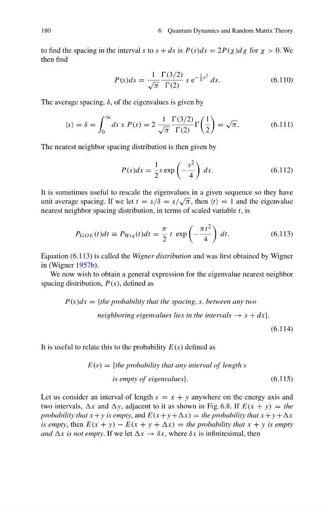
P (s)ds =
1
√
π
(3/2)
(2)
s e
−
1
4 s 2 ds.
(6.110)
The average spacing, δ, of the eigenvalues is given by
s = δ =
∞
0
ds s P (s) = 2
1
√
π
(3/2)
(2)
1
2
=
√
π.
(6.111)
The nearest neighbor spacing distribution is then given by
P (s)ds =
1
2
s exp
−
s 2
4
ds.
(6.112)
It is sometimes useful to rescale the eigenvalues in a given sequence so they have
unit average spacing. If we let t = s/δ = s/
√
π , then t = 1 and the eigenvalue
nearest neighbor spacing distribution, in terms of scaled variable t, is
P GOE (t)dt ≡ P W ig (t)dt =
π
2
t exp
−
πt 2
4
dt.
(6.113)
Equation (6.113) is called the Wigner distribution and was first obtained by Wigner
in (Wigner 1957b).
We now wish to obtain a general expression for the eigenvalue nearest neighbor
spacing distribution, P (s), defined as
P (s)ds = {the probability that the spacing, s, between any two
neighboring eigenvalues lies in the intervals → s + ds}.
(6.114)
It is useful to relate this to the probability E(s) defined as
E(s) = {the probability that any interval of length s
is empty of eigenvalues}.
(6.115)
Let us consider an interval of length s = x + y anywhere on the energy axis and
two intervals, x and y, adjacent to it as shown in Fig. 6.8. If E(x + y) = the
probability that x +y is empty, and E(x +y +x) = the probability that x +y +x
is empty, then E(x + y) − E(x + y + x) = the probability that x + y is empty
and x is not empty. If we let x → δx, where δx is infinitesimal, then
6 Quantum Dynamics and Random Matrix Theory
to find the spacing in the interval s to s + ds is P (s)ds = 2P (χ)dχ for χ > 0. We
then find
P (s)ds =
1
√
π
(3/2)
(2)
s e
−
1
4 s 2 ds.
(6.110)
The average spacing, δ, of the eigenvalues is given by
s = δ =
∞
0
ds s P (s) = 2
1
√
π
(3/2)
(2)
1
2
=
√
π.
(6.111)
The nearest neighbor spacing distribution is then given by
P (s)ds =
1
2
s exp
−
s 2
4
ds.
(6.112)
It is sometimes useful to rescale the eigenvalues in a given sequence so they have
unit average spacing. If we let t = s/δ = s/
√
π , then t = 1 and the eigenvalue
nearest neighbor spacing distribution, in terms of scaled variable t, is
P GOE (t)dt ≡ P W ig (t)dt =
π
2
t exp
−
πt 2
4
dt.
(6.113)
Equation (6.113) is called the Wigner distribution and was first obtained by Wigner
in (Wigner 1957b).
We now wish to obtain a general expression for the eigenvalue nearest neighbor
spacing distribution, P (s), defined as
P (s)ds = {the probability that the spacing, s, between any two
neighboring eigenvalues lies in the intervals → s + ds}.
(6.114)
It is useful to relate this to the probability E(s) defined as
E(s) = {the probability that any interval of length s
is empty of eigenvalues}.
(6.115)
Let us consider an interval of length s = x + y anywhere on the energy axis and
two intervals, x and y, adjacent to it as shown in Fig. 6.8. If E(x + y) = the
probability that x +y is empty, and E(x +y +x) = the probability that x +y +x
is empty, then E(x + y) − E(x + y + x) = the probability that x + y is empty
and x is not empty. If we let x → δx, where δx is infinitesimal, then