

6.4 Eigenvalue Statistics: Gaussian Orthogonal Ensemble
169
ln[P (x 1 , . . . , x N )] = C N −
1
2
N
i=1
x
2
i +
N
i>j =1
ln |x i − x j |,
(6.64)
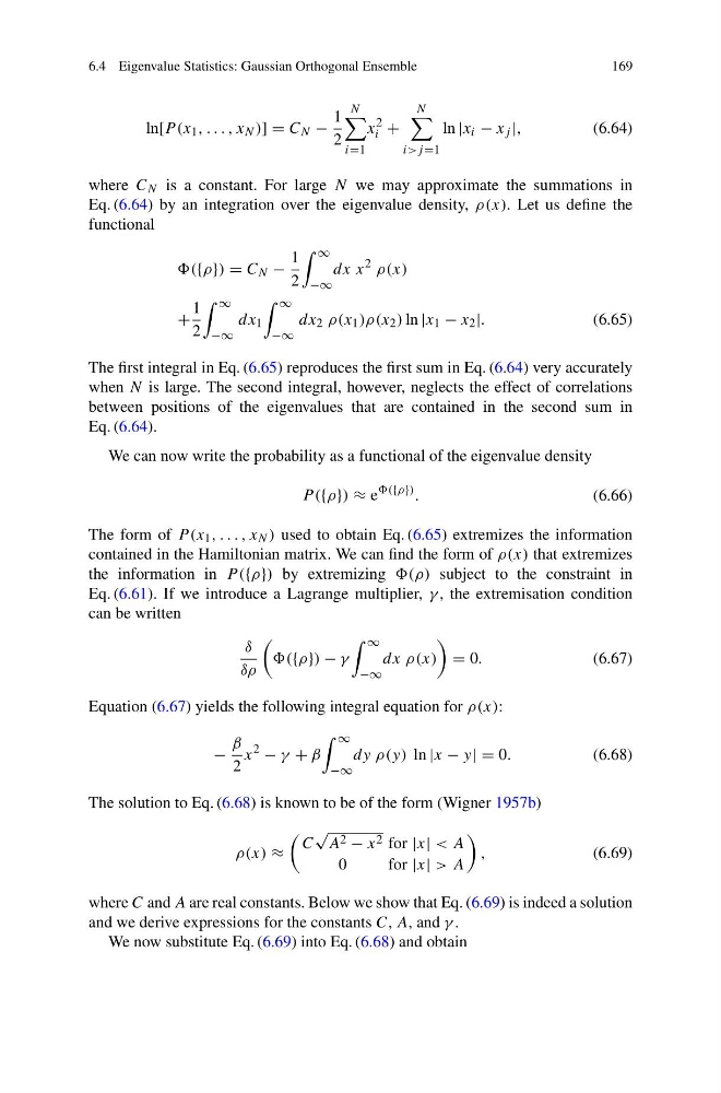
where C N is a constant. For large N we may approximate the summations in
Eq. (6.64) by an integration over the eigenvalue density, ρ(x). Let us define the
functional
({ρ}) = C N −
1
2
∞
−∞
dx x
2 ρ(x)
+
1
2
∞
−∞
dx 1
∞
−∞
dx 2 ρ(x 1 )ρ(x 2 ) ln |x 1 − x 2 |.
(6.65)
The first integral in Eq. (6.65) reproduces the first sum in Eq. (6.64) very accurately
when N is large. The second integral, however, neglects the effect of correlations
between positions of the eigenvalues that are contained in the second sum in
Eq. (6.64).
We can now write the probability as a functional of the eigenvalue density
P ({ρ}) ≈ e
({ρ}) .
(6.66)
The form of P (x 1 , . . . , x N ) used to obtain Eq. (6.65) extremizes the information
contained in the Hamiltonian matrix. We can find the form of ρ(x) that extremizes
the information in P ({ρ}) by extremizing subject to the constraint in
Eq. (6.61). If we introduce a Lagrange multiplier, γ , the extremisation condition
can be written
δ
δρ
({ρ}) − γ
∞
−∞
dx ρ(x)
= 0.
(6.67)
Equation (6.67) yields the following integral equation for ρ(x):
−
β
2
x
2
− γ + β
∞
−∞
dy ρ(y) ln |x − y| = 0.
(6.68)
The solution to Eq. (6.68) is known to be of the form (Wigner 1957b)
ρ(x) ≈
C
√
A 2 − x 2 for |x| < A
0
for|x| > A
,
(6.69)
where C and A are real constants. Below we show that Eq. (6.69) is indeed a solution
and we derive expressions for the constants C, A, and γ .
We now substitute Eq. (6.69) into Eq. (6.68) and obtain
169
ln[P (x 1 , . . . , x N )] = C N −
1
2
N
i=1
x
2
i +
N
i>j =1
ln |x i − x j |,
(6.64)
where C N is a constant. For large N we may approximate the summations in
Eq. (6.64) by an integration over the eigenvalue density, ρ(x). Let us define the
functional
({ρ}) = C N −
1
2
∞
−∞
dx x
2 ρ(x)
+
1
2
∞
−∞
dx 1
∞
−∞
dx 2 ρ(x 1 )ρ(x 2 ) ln |x 1 − x 2 |.
(6.65)
The first integral in Eq. (6.65) reproduces the first sum in Eq. (6.64) very accurately
when N is large. The second integral, however, neglects the effect of correlations
between positions of the eigenvalues that are contained in the second sum in
Eq. (6.64).
We can now write the probability as a functional of the eigenvalue density
P ({ρ}) ≈ e
({ρ}) .
(6.66)
The form of P (x 1 , . . . , x N ) used to obtain Eq. (6.65) extremizes the information
contained in the Hamiltonian matrix. We can find the form of ρ(x) that extremizes
the information in P ({ρ}) by extremizing subject to the constraint in
Eq. (6.61). If we introduce a Lagrange multiplier, γ , the extremisation condition
can be written
δ
δρ
({ρ}) − γ
∞
−∞
dx ρ(x)
= 0.
(6.67)
Equation (6.67) yields the following integral equation for ρ(x):
−
β
2
x
2
− γ + β
∞
−∞
dy ρ(y) ln |x − y| = 0.
(6.68)
The solution to Eq. (6.68) is known to be of the form (Wigner 1957b)
ρ(x) ≈
C
√
A 2 − x 2 for |x| < A
0
for|x| > A
,
(6.69)
where C and A are real constants. Below we show that Eq. (6.69) is indeed a solution
and we derive expressions for the constants C, A, and γ .
We now substitute Eq. (6.69) into Eq. (6.68) and obtain