

170
6 Quantum Dynamics and Random Matrix Theory
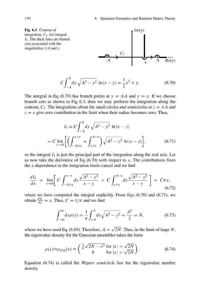
Fig. 6.3 Contour of
integration, C 1 , for integral
I 1 . The thick lines are branch
cuts associated with the
singularities ±A and x
C
A
−A
dy
A 2 − y 2 ln |x − y| =
1
2
x
2
+ γ.
(6.70)
The integral in Eq. (6.70) has branch points at y = ±A and y = x. If we choose
branch cuts as shown in Fig. 6.3, then we may perform the integration along the
contour, C 1 . The integrations about the small circles and semicircles at z = ±A and
z = x give zero contribution in the limit when their radius becomes zero. Thus,
I 1 ≡ C
A
−A
dy
A 2 − y 2 ln |x − y|
= C lim
x−
−A+
+
A−
x+
A 2 − y 2 ln |x − y|
,
(6.71)
so the integral I 1 is just the principal part of the integration along the real axis. Let
us now take the derivative of Eq. (6.70) with respect to x. The contributions from
the x-dependence in the integration limits cancel and we find
dI 1
dx
= lim
C
x−
−A+
dy
A 2 − y 2
x − y
+ C
A−
x+
dy
A 2 − y 2
x − y
= Cπx,
(6.72)
where we have computed the integral explicitly. From Eqs. (6.70) and (6.71), we
obtain
dI 1
dx = x. Thus, C = 1/π and we find
∞
−∞
dyρ(y) =
1
π
A
=A
dy
A 2 − y 2 =
A 2
2
= N,
(6.73)
where we have used Eq. (6.69). Therefore, A =
√
2N . Thus, in the limit of large N,
the eigenvalue density for the Gaussian ensembles takes the form
ρ(x)≈ρ wig (x) ≈
1
π
√
2N − x 2 for |x| <
√
2N
0
for|x| >
√
2N
.
(6.74)
Equation (6.74) is called the Wigner semicircle law for the eigenvalue number
density.
6 Quantum Dynamics and Random Matrix Theory
Fig. 6.3 Contour of
integration, C 1 , for integral
I 1 . The thick lines are branch
cuts associated with the
singularities ±A and x
C
A
−A
dy
A 2 − y 2 ln |x − y| =
1
2
x
2
+ γ.
(6.70)
The integral in Eq. (6.70) has branch points at y = ±A and y = x. If we choose
branch cuts as shown in Fig. 6.3, then we may perform the integration along the
contour, C 1 . The integrations about the small circles and semicircles at z = ±A and
z = x give zero contribution in the limit when their radius becomes zero. Thus,
I 1 ≡ C
A
−A
dy
A 2 − y 2 ln |x − y|
= C lim
x−
−A+
+
A−
x+
A 2 − y 2 ln |x − y|
,
(6.71)
so the integral I 1 is just the principal part of the integration along the real axis. Let
us now take the derivative of Eq. (6.70) with respect to x. The contributions from
the x-dependence in the integration limits cancel and we find
dI 1
dx
= lim
C
x−
−A+
dy
A 2 − y 2
x − y
+ C
A−
x+
dy
A 2 − y 2
x − y
= Cπx,
(6.72)
where we have computed the integral explicitly. From Eqs. (6.70) and (6.71), we
obtain
dI 1
dx = x. Thus, C = 1/π and we find
∞
−∞
dyρ(y) =
1
π
A
=A
dy
A 2 − y 2 =
A 2
2
= N,
(6.73)
where we have used Eq. (6.69). Therefore, A =
√
2N . Thus, in the limit of large N,
the eigenvalue density for the Gaussian ensembles takes the form
ρ(x)≈ρ wig (x) ≈
1
π
√
2N − x 2 for |x| <
√
2N
0
for|x| >
√
2N
.
(6.74)
Equation (6.74) is called the Wigner semicircle law for the eigenvalue number
density.