

168
6 Quantum Dynamics and Random Matrix Theory
ρ N (x) = = ˆ
ρ(x) N =
all
dx 1 . . .
all
dx N ˆ
ρ(x) P N (x 1 , . . . , x N )
= N
all
dx 1 . . .
all
dx N δ(x − x 1 )P N (x 1 , . . . , x N ) = R N (x) = T N (x),
(6.60)
where
all dx j =
∞
−∞ dx j .
The average number of eigenvalues in the energy interval x→x +dx is ρ N (x)dx,
where
∞
−∞
ρ N (x)dx = N.
(6.61)
If we use Eq. (6.49), we can write
ρ N (x) ˆ
1 = T N (x) ˆ
1 = ¯
σ N (x, x),
(6.62)
where ˆ
1 =
1 0
0 1
. If we use Eq. (6.53), the eigenvalue density for the Gaussian
orthogonal ensemble (GOE) is
ρ N (x) =
N
2 −1
k=0
φ 2k (x)φ 2k (x) − φ
2k (x)
x
0
dtφ 2k (t)
.
(6.63)
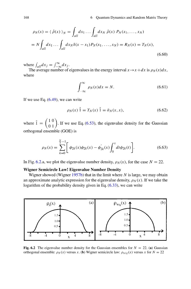
In Fig. 6.2.a, we plot the eigenvalue number density, ρ N (x), for the case N = 22.
Wigner Semicircle Law! Eigenvalue Number Density
Wigner showed (Wigner 1957b) that in the limit where N is large, we may obtain
an approximate analytic expression for the eigenvalue density, ρ N (x). If we take the
logarithm of the probability density given in Eq. (6.33), we can write
Fig. 6.2 The eigenvalue number density for the Gaussian ensembles for N = 22. (a) Gaussian
orthogonal ensemble: ρ N (x) versus x. (b) Wigner semicircle law: ρ wig (x) versus x for N = 22
6 Quantum Dynamics and Random Matrix Theory
ρ N (x) = = ˆ
ρ(x) N =
all
dx 1 . . .
all
dx N ˆ
ρ(x) P N (x 1 , . . . , x N )
= N
all
dx 1 . . .
all
dx N δ(x − x 1 )P N (x 1 , . . . , x N ) = R N (x) = T N (x),
(6.60)
where
all dx j =
∞
−∞ dx j .
The average number of eigenvalues in the energy interval x→x +dx is ρ N (x)dx,
where
∞
−∞
ρ N (x)dx = N.
(6.61)
If we use Eq. (6.49), we can write
ρ N (x) ˆ
1 = T N (x) ˆ
1 = ¯
σ N (x, x),
(6.62)
where ˆ
1 =
1 0
0 1
. If we use Eq. (6.53), the eigenvalue density for the Gaussian
orthogonal ensemble (GOE) is
ρ N (x) =
N
2 −1
k=0
φ 2k (x)φ 2k (x) − φ
2k (x)
x
0
dtφ 2k (t)
.
(6.63)
In Fig. 6.2.a, we plot the eigenvalue number density, ρ N (x), for the case N = 22.
Wigner Semicircle Law! Eigenvalue Number Density
Wigner showed (Wigner 1957b) that in the limit where N is large, we may obtain
an approximate analytic expression for the eigenvalue density, ρ N (x). If we take the
logarithm of the probability density given in Eq. (6.33), we can write
Fig. 6.2 The eigenvalue number density for the Gaussian ensembles for N = 22. (a) Gaussian
orthogonal ensemble: ρ N (x) versus x. (b) Wigner semicircle law: ρ wig (x) versus x for N = 22