

146
5 Arnol’d Diffusion
5.5.2 Arnol’d Diffusion
The Hamiltonian in Eq. (5.17) can be written in a time-independent form if we
replace the time by an angle variable φ 3 = ωt in Eq. (5.17) and include the
corresponding action, I 3 . The Hamiltonian then takes the form
H = p
2
x + p
2
y + ωI 3 +
U
2
cos
2 (x) +
U
2
cos
2 (y) + b
U
2
cos(x)cos(y)
+
U
2
cos(2φ 3 )cos
2 (x) +
U
2
cos(2φ 3 )cos
2 (y)
+b
U
2
cos(2φ 3 )cos(x)cos(y).
(5.22)
If one writes Hamilton’s equations for this system, one finds that φ 3 (t) = ωt and
I 3 = −H (t)/ω, so no new dynamics is involved. This Hamiltonian, when written in
terms of action-angle variables (see Eq. (5.20)), contains all harmonics at first order
in the parameter b, which is the parameter governing the character of the Arnol’d
diffusion.
We can use the Walker-Ford method discussed in Chap. 2 to obtain a very rough
estimate of the value of b for which the Nekhoroshev regime transitions to the
Chirikov regime. For the rotation-version of the Hamiltonian in Eq. (5.20), we
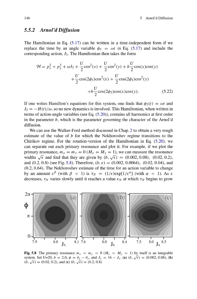
can separate out each primary resonance and plot it. For example, if we plot the
primary resonance, m x = m y = 0 (M x = M y = 1), we can measure the resonance
widths
√
and find that they are given by (b,
√
) = (0.002, 0.08), (0.02, 0.2),
and (0.2, 0.8) (see Fig. 5.8). Therefore, (b, ) = (0.002, 0.0064), (0.02, 0.04), and
(0.2, 0.64). The Nekhoroshev estimate of the time for an action variable to change
by an amount β (with β < 1) is τ N = (1//)exp[1// α ] (with α < 1). As
decreases, τ N varies slowly until it reaches a value N at which τ N begins to grow
Fig. 5.8 The primary resonance m x = m y = 0 (M x = M y = 1) by itself is an integrable
system. Set U=20, b = 2.0, φ = θ x − θ y , and J y = 16 − J x . (a) (b,
√
) = (0.002, 0.08), (b)
(b,
√
) = (0.02, 0.2), and (c) (b,
√
) = (0.2, 0.8)
5 Arnol’d Diffusion
5.5.2 Arnol’d Diffusion
The Hamiltonian in Eq. (5.17) can be written in a time-independent form if we
replace the time by an angle variable φ 3 = ωt in Eq. (5.17) and include the
corresponding action, I 3 . The Hamiltonian then takes the form
H = p
2
x + p
2
y + ωI 3 +
U
2
cos
2 (x) +
U
2
cos
2 (y) + b
U
2
cos(x)cos(y)
+
U
2
cos(2φ 3 )cos
2 (x) +
U
2
cos(2φ 3 )cos
2 (y)
+b
U
2
cos(2φ 3 )cos(x)cos(y).
(5.22)
If one writes Hamilton’s equations for this system, one finds that φ 3 (t) = ωt and
I 3 = −H (t)/ω, so no new dynamics is involved. This Hamiltonian, when written in
terms of action-angle variables (see Eq. (5.20)), contains all harmonics at first order
in the parameter b, which is the parameter governing the character of the Arnol’d
diffusion.
We can use the Walker-Ford method discussed in Chap. 2 to obtain a very rough
estimate of the value of b for which the Nekhoroshev regime transitions to the
Chirikov regime. For the rotation-version of the Hamiltonian in Eq. (5.20), we
can separate out each primary resonance and plot it. For example, if we plot the
primary resonance, m x = m y = 0 (M x = M y = 1), we can measure the resonance
widths
√
and find that they are given by (b,
√
) = (0.002, 0.08), (0.02, 0.2),
and (0.2, 0.8) (see Fig. 5.8). Therefore, (b, ) = (0.002, 0.0064), (0.02, 0.04), and
(0.2, 0.64). The Nekhoroshev estimate of the time for an action variable to change
by an amount β (with β < 1) is τ N = (1//)exp[1// α ] (with α < 1). As
decreases, τ N varies slowly until it reaches a value N at which τ N begins to grow
Fig. 5.8 The primary resonance m x = m y = 0 (M x = M y = 1) by itself is an integrable
system. Set U=20, b = 2.0, φ = θ x − θ y , and J y = 16 − J x . (a) (b,
√
) = (0.002, 0.08), (b)
(b,
√
) = (0.02, 0.2), and (c) (b,
√
) = (0.2, 0.8)