

5.5 Arnol’d Diffusion in an Optical Lattice
147
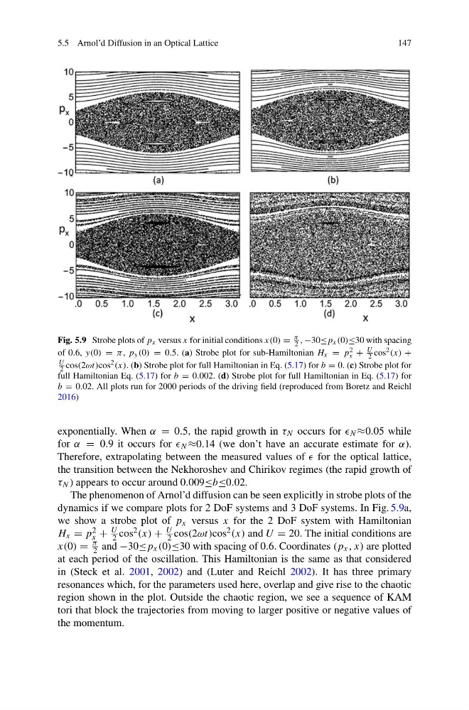
Fig. 5.9 Strobe plots of p x versus x for initial conditions x(0) =
π
2 , −30≤p x (0)≤30 with spacing
of 0.6, y(0) = π , p y (0) = 0.5. (a) Strobe plot for sub-Hamiltonian H x = p 2
x +
U
2 cos 2 (x) +
U
2 cos(2ωt)cos 2 (x). (b) Strobe plot for full Hamiltonian in Eq. (5.17) for b = 0. (c) Strobe plot for
full Hamiltonian Eq. (5.17) for b = 0.002. (d) Strobe plot for full Hamiltonian in Eq. (5.17) for
b = 0.02. All plots run for 2000 periods of the driving field (reproduced from Boretz and Reichl
2016)
exponentially. When α = 0.5, the rapid growth in τ N occurs for N ≈0.05 while
for α = 0.9 it occurs for N ≈0.14 (we don’t have an accurate estimate for α).
Therefore, extrapolating between the measured values of for the optical lattice,
the transition between the Nekhoroshev and Chirikov regimes (the rapid growth of
τ N ) appears to occur around 0.009≤b≤0.02.
The phenomenon of Arnol’d diffusion can be seen explicitly in strobe plots of the
dynamics if we compare plots for 2 DoF systems and 3 DoF systems. In Fig. 5.9a,
we show a strobe plot of p x versus x for the 2 DoF system with Hamiltonian
H x = p 2
x +
U
2 cos 2 (x) +
U
2 cos(2ωt)cos 2 (x) and U = 20. The initial conditions are
x(0) =
π
2 and −30≤p x (0)≤30 with spacing of 0.6. Coordinates (p x , x) are plotted
at each period of the oscillation. This Hamiltonian is the same as that considered
in (Steck et al. 2001, 2002) and (Luter and Reichl 2002). It has three primary
resonances which, for the parameters used here, overlap and give rise to the chaotic
region shown in the plot. Outside the chaotic region, we see a sequence of KAM
tori that block the trajectories from moving to larger positive or negative values of
the momentum.
147
Fig. 5.9 Strobe plots of p x versus x for initial conditions x(0) =
π
2 , −30≤p x (0)≤30 with spacing
of 0.6, y(0) = π , p y (0) = 0.5. (a) Strobe plot for sub-Hamiltonian H x = p 2
x +
U
2 cos 2 (x) +
U
2 cos(2ωt)cos 2 (x). (b) Strobe plot for full Hamiltonian in Eq. (5.17) for b = 0. (c) Strobe plot for
full Hamiltonian Eq. (5.17) for b = 0.002. (d) Strobe plot for full Hamiltonian in Eq. (5.17) for
b = 0.02. All plots run for 2000 periods of the driving field (reproduced from Boretz and Reichl
2016)
exponentially. When α = 0.5, the rapid growth in τ N occurs for N ≈0.05 while
for α = 0.9 it occurs for N ≈0.14 (we don’t have an accurate estimate for α).
Therefore, extrapolating between the measured values of for the optical lattice,
the transition between the Nekhoroshev and Chirikov regimes (the rapid growth of
τ N ) appears to occur around 0.009≤b≤0.02.
The phenomenon of Arnol’d diffusion can be seen explicitly in strobe plots of the
dynamics if we compare plots for 2 DoF systems and 3 DoF systems. In Fig. 5.9a,
we show a strobe plot of p x versus x for the 2 DoF system with Hamiltonian
H x = p 2
x +
U
2 cos 2 (x) +
U
2 cos(2ωt)cos 2 (x) and U = 20. The initial conditions are
x(0) =
π
2 and −30≤p x (0)≤30 with spacing of 0.6. Coordinates (p x , x) are plotted
at each period of the oscillation. This Hamiltonian is the same as that considered
in (Steck et al. 2001, 2002) and (Luter and Reichl 2002). It has three primary
resonances which, for the parameters used here, overlap and give rise to the chaotic
region shown in the plot. Outside the chaotic region, we see a sequence of KAM
tori that block the trajectories from moving to larger positive or negative values of
the momentum.