

5.5 Arnol’d Diffusion in an Optical Lattice
143
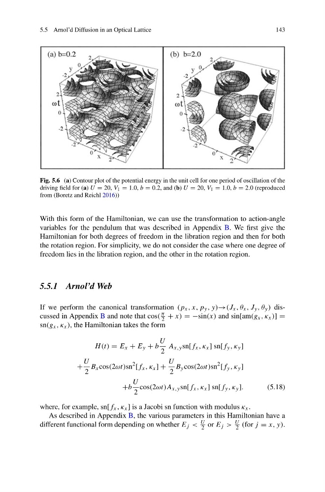
Fig. 5.6 (a) Contour plot of the potential energy in the unit cell for one period of oscillation of the
driving field for (a) U = 20, V 1 = 1.0, b = 0.2, and (b) U = 20, V 1 = 1.0, b = 2.0 (reproduced
from (Boretz and Reichl 2016))
With this form of the Hamiltonian, we can use the transformation to action-angle
variables for the pendulum that was described in Appendix B. We first give the
Hamiltonian for both degrees of freedom in the libration region and then for both
the rotation region. For simplicity, we do not consider the case where one degree of
freedom lies in the libration region, and the other in the rotation region.
5.5.1 Arnol’d Web
If we perform the canonical transformation (p x , x, p y , y)→(J x , θ x , J y , θ y ) discussed in Appendix B and note that cos(
π
2 + x) = −sin(x) and sin[am(g x , κ x )] =
sn(g x , κ x ), the Hamiltonian takes the form
H (t) = E x + E y + b
U
2
A x,y sn[f x , κ x ] sn[f y , κ y ]
+
U
2
B x cos(2ωt)sn
2
[f x , κ x ] +
U
2
B y cos(2ωt)sn
2
[f y , κ y ]
+b
U
2
cos(2ωt)A x,y sn[f x , κ x ] sn[f y , κ y ].
(5.18)
where, for example, sn[f x , κ x ] is a Jacobi sn function with modulus κ x .
As described in Appendix B, the various parameters in this Hamiltonian have a
different functional form depending on whether E j <
U
2 or E j >
U
2 (for j = x, y).
143
Fig. 5.6 (a) Contour plot of the potential energy in the unit cell for one period of oscillation of the
driving field for (a) U = 20, V 1 = 1.0, b = 0.2, and (b) U = 20, V 1 = 1.0, b = 2.0 (reproduced
from (Boretz and Reichl 2016))
With this form of the Hamiltonian, we can use the transformation to action-angle
variables for the pendulum that was described in Appendix B. We first give the
Hamiltonian for both degrees of freedom in the libration region and then for both
the rotation region. For simplicity, we do not consider the case where one degree of
freedom lies in the libration region, and the other in the rotation region.
5.5.1 Arnol’d Web
If we perform the canonical transformation (p x , x, p y , y)→(J x , θ x , J y , θ y ) discussed in Appendix B and note that cos(
π
2 + x) = −sin(x) and sin[am(g x , κ x )] =
sn(g x , κ x ), the Hamiltonian takes the form
H (t) = E x + E y + b
U
2
A x,y sn[f x , κ x ] sn[f y , κ y ]
+
U
2
B x cos(2ωt)sn
2
[f x , κ x ] +
U
2
B y cos(2ωt)sn
2
[f y , κ y ]
+b
U
2
cos(2ωt)A x,y sn[f x , κ x ] sn[f y , κ y ].
(5.18)
where, for example, sn[f x , κ x ] is a Jacobi sn function with modulus κ x .
As described in Appendix B, the various parameters in this Hamiltonian have a
different functional form depending on whether E j <
U
2 or E j >
U
2 (for j = x, y).