

142
5 Arnol’d Diffusion
We want to examine the behavior of the atoms in this lattice, both in the static
case and with increasing amplitude of the time-periodic modulation of the optical
lattice amplitude. To this end, we generalize this Hamiltonian and write it in the
form
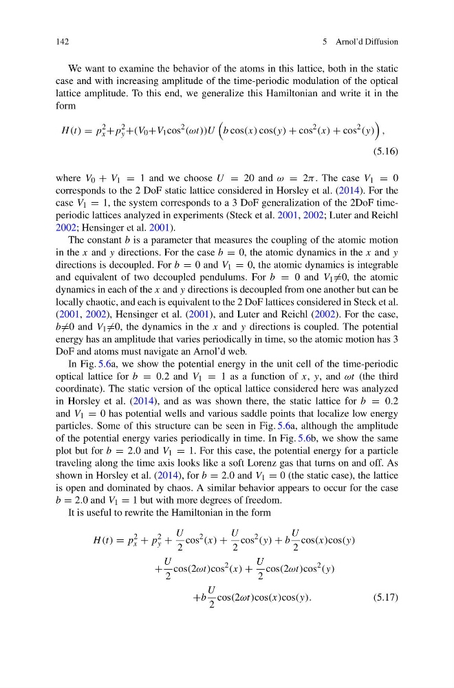
H (t) = p
2
x +p
2
y +(V 0 +V 1 cos
2 (ωt))U
b cos(x) cos(y) + cos
2 (x) + cos
2 (y)
,
(5.16)
where V 0 + V 1 = 1 and we choose U = 20 and ω = 2π . The case V 1 = 0
corresponds to the 2 DoF static lattice considered in Horsley et al. (2014). For the
case V 1 = 1, the system corresponds to a 3 DoF generalization of the 2DoF timeperiodic lattices analyzed in experiments (Steck et al. 2001, 2002; Luter and Reichl
2002; Hensinger et al. 2001).
The constant b is a parameter that measures the coupling of the atomic motion
in the x and y directions. For the case b = 0, the atomic dynamics in the x and y
directions is decoupled. For b = 0 and V 1 = 0, the atomic dynamics is integrable
and equivalent of two decoupled pendulums. For b = 0 and V 1 =0, the atomic
dynamics in each of the x and y directions is decoupled from one another but can be
locally chaotic, and each is equivalent to the 2 DoF lattices considered in Steck et al.
(2001, 2002), Hensinger et al. (2001), and Luter and Reichl (2002). For the case,
b =0 and V 1 =0, the dynamics in the x and y directions is coupled. The potential
energy has an amplitude that varies periodically in time, so the atomic motion has 3
DoF and atoms must navigate an Arnol’d web.
In Fig. 5.6a, we show the potential energy in the unit cell of the time-periodic
optical lattice for b = 0.2 and V 1 = 1 as a function of x, y, and ωt (the third
coordinate). The static version of the optical lattice considered here was analyzed
in Horsley et al. (2014), and as was shown there, the static lattice for b = 0.2
and V 1 = 0 has potential wells and various saddle points that localize low energy
particles. Some of this structure can be seen in Fig. 5.6a, although the amplitude
of the potential energy varies periodically in time. In Fig. 5.6b, we show the same
plot but for b = 2.0 and V 1 = 1. For this case, the potential energy for a particle
traveling along the time axis looks like a soft Lorenz gas that turns on and off. As
shown in Horsley et al. (2014), for b = 2.0 and V 1 = 0 (the static case), the lattice
is open and dominated by chaos. A similar behavior appears to occur for the case
b = 2.0 and V 1 = 1 but with more degrees of freedom.
It is useful to rewrite the Hamiltonian in the form
H (t) = p
2
x + p
2
y +
U
2
cos
2 (x) +
U
2
cos
2 (y) + b
U
2
cos(x)cos(y)
+
U
2
cos(2ωt)cos
2 (x) +
U
2
cos(2ωt)cos
2 (y)
+b
U
2
cos(2ωt)cos(x)cos(y).
(5.17)
5 Arnol’d Diffusion
We want to examine the behavior of the atoms in this lattice, both in the static
case and with increasing amplitude of the time-periodic modulation of the optical
lattice amplitude. To this end, we generalize this Hamiltonian and write it in the
form
H (t) = p
2
x +p
2
y +(V 0 +V 1 cos
2 (ωt))U
b cos(x) cos(y) + cos
2 (x) + cos
2 (y)
,
(5.16)
where V 0 + V 1 = 1 and we choose U = 20 and ω = 2π . The case V 1 = 0
corresponds to the 2 DoF static lattice considered in Horsley et al. (2014). For the
case V 1 = 1, the system corresponds to a 3 DoF generalization of the 2DoF timeperiodic lattices analyzed in experiments (Steck et al. 2001, 2002; Luter and Reichl
2002; Hensinger et al. 2001).
The constant b is a parameter that measures the coupling of the atomic motion
in the x and y directions. For the case b = 0, the atomic dynamics in the x and y
directions is decoupled. For b = 0 and V 1 = 0, the atomic dynamics is integrable
and equivalent of two decoupled pendulums. For b = 0 and V 1 =0, the atomic
dynamics in each of the x and y directions is decoupled from one another but can be
locally chaotic, and each is equivalent to the 2 DoF lattices considered in Steck et al.
(2001, 2002), Hensinger et al. (2001), and Luter and Reichl (2002). For the case,
b =0 and V 1 =0, the dynamics in the x and y directions is coupled. The potential
energy has an amplitude that varies periodically in time, so the atomic motion has 3
DoF and atoms must navigate an Arnol’d web.
In Fig. 5.6a, we show the potential energy in the unit cell of the time-periodic
optical lattice for b = 0.2 and V 1 = 1 as a function of x, y, and ωt (the third
coordinate). The static version of the optical lattice considered here was analyzed
in Horsley et al. (2014), and as was shown there, the static lattice for b = 0.2
and V 1 = 0 has potential wells and various saddle points that localize low energy
particles. Some of this structure can be seen in Fig. 5.6a, although the amplitude
of the potential energy varies periodically in time. In Fig. 5.6b, we show the same
plot but for b = 2.0 and V 1 = 1. For this case, the potential energy for a particle
traveling along the time axis looks like a soft Lorenz gas that turns on and off. As
shown in Horsley et al. (2014), for b = 2.0 and V 1 = 0 (the static case), the lattice
is open and dominated by chaos. A similar behavior appears to occur for the case
b = 2.0 and V 1 = 1 but with more degrees of freedom.
It is useful to rewrite the Hamiltonian in the form
H (t) = p
2
x + p
2
y +
U
2
cos
2 (x) +
U
2
cos
2 (y) + b
U
2
cos(x)cos(y)
+
U
2
cos(2ωt)cos
2 (x) +
U
2
cos(2ωt)cos
2 (y)
+b
U
2
cos(2ωt)cos(x)cos(y).
(5.17)