

136
5 Arnol’d Diffusion
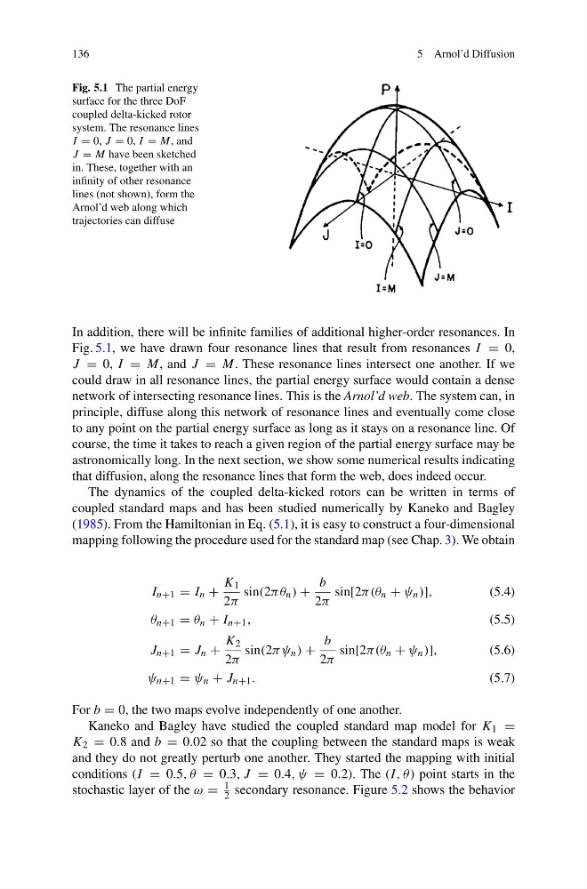
Fig. 5.1 The partial energy
surface for the three DoF
coupled delta-kicked rotor
system. The resonance lines
I = 0, J = 0, I = M, and
J = M have been sketched
in. These, together with an
infinity of other resonance
lines (not shown), form the
Arnol’d web along which
trajectories can diffuse
In addition, there will be infinite families of additional higher-order resonances. In
Fig. 5.1, we have drawn four resonance lines that result from resonances I = 0,
J = 0, I = M, and J = M. These resonance lines intersect one another. If we
could draw in all resonance lines, the partial energy surface would contain a dense
network of intersecting resonance lines. This is the Arnol’d web. The system can, in
principle, diffuse along this network of resonance lines and eventually come close
to any point on the partial energy surface as long as it stays on a resonance line. Of
course, the time it takes to reach a given region of the partial energy surface may be
astronomically long. In the next section, we show some numerical results indicating
that diffusion, along the resonance lines that form the web, does indeed occur.
The dynamics of the coupled delta-kicked rotors can be written in terms of
coupled standard maps and has been studied numerically by Kaneko and Bagley
(1985). From the Hamiltonian in Eq. (5.1), it is easy to construct a four-dimensional
mapping following the procedure used for the standard map (see Chap. 3). We obtain
I n+1 = I n +
K 1
2π
sin(2πθ n ) +
b
2π
sin[2π(θ n + ψ n )],
(5.4)
θ n+1 = θ n + I n+1 ,
(5.5)
J n+1 = J n +
K 2
2π
sin(2πψ n ) +
b
2π
sin[2π(θ n + ψ n )],
(5.6)
ψ n+1 = ψ n + J n+1 .
(5.7)
For b = 0, the two maps evolve independently of one another.
Kaneko and Bagley have studied the coupled standard map model for K 1 =
K 2 = 0.8 and b = 0.02 so that the coupling between the standard maps is weak
and they do not greatly perturb one another. They started the mapping with initial
conditions (I = 0.5, θ = 0.3, J = 0.4, ψ = 0.2). The (I, θ) point starts in the
stochastic layer of the ω =
1
2 secondary resonance. Figure 5.2 shows the behavior
5 Arnol’d Diffusion
Fig. 5.1 The partial energy
surface for the three DoF
coupled delta-kicked rotor
system. The resonance lines
I = 0, J = 0, I = M, and
J = M have been sketched
in. These, together with an
infinity of other resonance
lines (not shown), form the
Arnol’d web along which
trajectories can diffuse
In addition, there will be infinite families of additional higher-order resonances. In
Fig. 5.1, we have drawn four resonance lines that result from resonances I = 0,
J = 0, I = M, and J = M. These resonance lines intersect one another. If we
could draw in all resonance lines, the partial energy surface would contain a dense
network of intersecting resonance lines. This is the Arnol’d web. The system can, in
principle, diffuse along this network of resonance lines and eventually come close
to any point on the partial energy surface as long as it stays on a resonance line. Of
course, the time it takes to reach a given region of the partial energy surface may be
astronomically long. In the next section, we show some numerical results indicating
that diffusion, along the resonance lines that form the web, does indeed occur.
The dynamics of the coupled delta-kicked rotors can be written in terms of
coupled standard maps and has been studied numerically by Kaneko and Bagley
(1985). From the Hamiltonian in Eq. (5.1), it is easy to construct a four-dimensional
mapping following the procedure used for the standard map (see Chap. 3). We obtain
I n+1 = I n +
K 1
2π
sin(2πθ n ) +
b
2π
sin[2π(θ n + ψ n )],
(5.4)
θ n+1 = θ n + I n+1 ,
(5.5)
J n+1 = J n +
K 2
2π
sin(2πψ n ) +
b
2π
sin[2π(θ n + ψ n )],
(5.6)
ψ n+1 = ψ n + J n+1 .
(5.7)
For b = 0, the two maps evolve independently of one another.
Kaneko and Bagley have studied the coupled standard map model for K 1 =
K 2 = 0.8 and b = 0.02 so that the coupling between the standard maps is weak
and they do not greatly perturb one another. They started the mapping with initial
conditions (I = 0.5, θ = 0.3, J = 0.4, ψ = 0.2). The (I, θ) point starts in the
stochastic layer of the ω =
1
2 secondary resonance. Figure 5.2 shows the behavior